

Naive Bayes classifier belongs to a family of probabilistic classifiers that are built upon the Bayes theorem. In naive Bayes classifiers, the number of model parameters increases linearly with the number of features. Moreover, it’s trained by evaluating a closed-form expression, i.e., a mathematical expression that can be evaluated using finite steps and has one definite solution. This means that naive Bayes classifiers train in linear time compared to the quadratic or cubic time of other iterative approximation based approaches. These two factors make naive Bayes classifiers highly scalable. In this article, we’ll go through the Bayes theorem, ‘make some assumptions’ and then implement a naive Bayes classifier from scratch.
Bayes Theorem
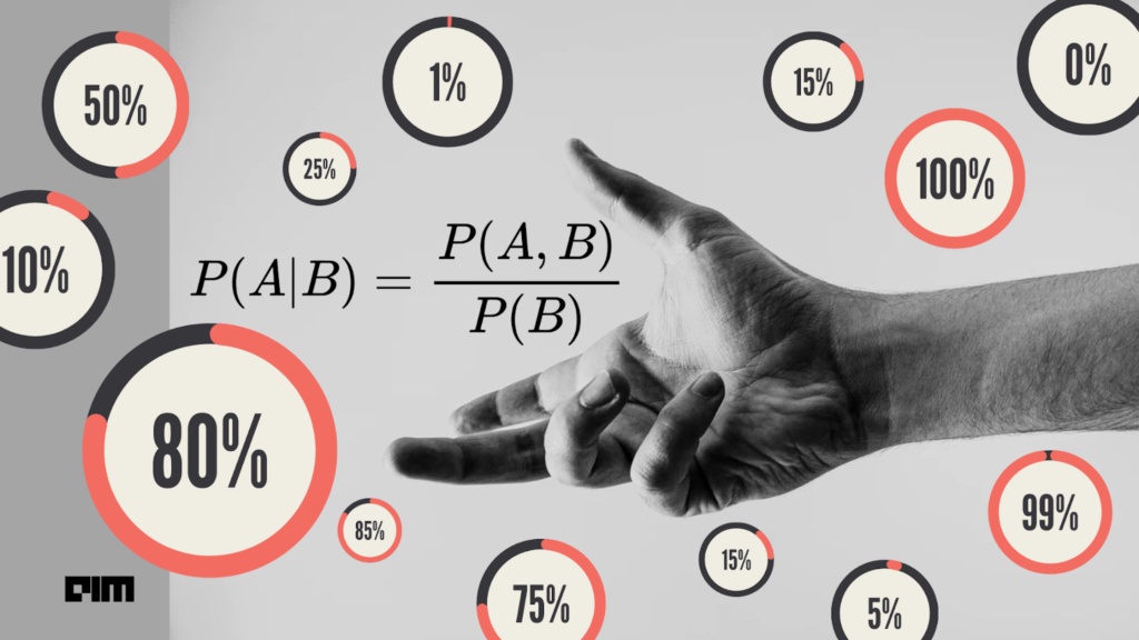
Bayes theorem is one of the most important formulas in all probability. It’s an essential tool for scientific discovery and for creating AI systems; it has also been used to find century-old treasures. It is formulated as

But what does that mean? Let’s understand it with the help of a puzzle taken from Kahneman and Tversky’s Experiments:
“Steve is very shy and withdrawn, invariably helpful but with very little interest in people or in the world of reality. A meek and tidy soul, he has a need for order and structure and a passion for detail.”
Given the above description, do you think Steve is more likely to be a librarian or a farmer? The majority of people immediately conclude that Steve must be a librarian since he fits their idea of a librarian. However, as we see the whole picture, we see that there are twenty times as many farmers as librarians (in the United States). Most people aren’t aware of this statistic and hence can’t make an accurate prediction, and that’s okay. Also, that’s beside the point of this article. However, if you want to learn why we act irrationally and make assumptions like this, I wholeheartedly recommend reading Kahneman’s Thinking Fast and Slow.
Back to Bayes theorem, to model this puzzle more accurately, let’s start by creating create a representative sample of 420 people, 20 librarians and 400 farmers. And let’s say your intuition is that roughly 50% of librarians would fit that description, and 10% of farmers would. So the probability of a random person fitting this description being a librarian becomes 0.2 (10/50). So even if you think a librarian is five times as likely as a farmer to fit this description, that’s not enough to overcome the fact that there are way more farmers.
This new evidence doesn’t necessarily overrule your past belief but rather updates it. And this is precisely what the Bayes theorem models. The first relevant number is the probability that your beliefs hold true before considering the new evidence. Using the ratio of farmers to librarians in the general population, this came out to be 1/5 in our example. This is known as the prior P(H). In addition to this, we need to consider the proportion of librarians that fit this description; the probability we would see the evidence given that the hypothesis is true, P(E|H). In the context of the Bayes theorem, this value is called the ‘likelihood’. This represents a limited view of your initial hypothesis.
Similarly, we need to consider how much of the farmer’s side of the sample space make up the evidence; the probability of seeing the evidence given that your beliefs don’t hold true P(E|H’). Using these notations, the accurate probability of your beliefs being right given the evidence, P(H|E), also called the posterior probability, can be formulated as:

Where N is the sample size. In our example, this expression evaluates to 1/5. The sample size gets cancelled out; this gives us:

This gets further simplified to:
This is the original Bayes theorem that we started with. I hope this illustrated the core point of the Bayes theorem representing a changing belief system, not just a bunch of independent probabilities.
Assumptions Made by Naive Bayes Classifiers
The naive Bayes classifier is called ‘naive’ because it makes the assumption that all features are independent of each other. Another assumption that it makes is that the values of the features are normally (Gaussian) distributed. Using these assumptions, the original Bayes theorem is modified and transformed into a simpler form that is relevant for solving learning problems. We start with

where,

And because the features are considered independent, we can breakdown P(X|y)

For classification tasks, we want to select the class with the highest probability, so we choose y, which is

And P(X) is common to all classes and will not change their final ranks; hence it can be excluded from the equation.

A lot of these probabilities will be small numbers; multiplying them can cause overflow problems, so we apply the log function.

And that’s the equation naive Bayes classifiers use to make predictions, now let’s implement one.
Implementing a Naive Bayes Classifier from Scratch
Create a function that calculates the prior probability, P(H), mean and variance of each class. The mean and variance are later used to calculate the likelihood, P(E|H), using the Gaussian distribution.
 import numpy as np
 class GaussianNaiveBayes:
     def fit(self, X, y):
         n_samples, n_features = X.shape
         self._classes = np.unique(y)
         n_classes = len(self._classes)
         self._mean = np.zeros((n_classes, n_features), dtype=np.float64)
         self._var = np.zeros((n_classes, n_features), dtype=np.float64)
         self._priors =  np.zeros(n_classes, dtype=np.float64)

         # calculating the mean, variance and prior P(H) for each class
         for i, c in enumerate(self._classes):
             X_for_class_c = X[y==c]
             self._mean[i, :] = X_for_class_c.mean(axis=0)
             self._var[i, :] = X_for_class_c.var(axis=0)
             self._priors[i] = X_for_class_c.shape[0] / float(n_samples)
Write a function for calculating the likelihood, P(E|H), of data X given the mean and variance
     def _calculate_likelihood(self, class_idx, x):
         mean = self._mean[class_idx]
         var = self._var[class_idx]
         num = np.exp(- (x-mean)**2 / (2 * var))
         denom = np.sqrt(2 * np.pi * var)
         return num / denom
And finally, write the methods for making classifications by calculating the posterior probability, P(H|E), of the classes
     def predict(self, X):
         y_pred = [self._classify_sample(x) for x in X]
         return np.array(y_pred)

     def _classify_sample(self, x):
         posteriors = []
         # calculating posterior probability for each class
         for i, c in enumerate(self._classes):
             prior = np.log(self._priors[i])
             posterior = np.sum(np.log(self._calculate_likelihood(i, x)))
             posterior = prior + posterior
             posteriors.append(posterior)
         # return the class with highest posterior probability
         return self._classes[np.argmax(posteriors)]
Now let’s test our naive Bayes classifier and compare it with scikit-learn’s implementation.
 from sklearn.model_selection import train_test_split
 from sklearn.metrics import accuracy_score
 from sklearn import datasets
 import time

 X, y = datasets.make_classification(n_samples=1000, n_features=20, n_classes=2, random_state=42)
 X_train, X_test, y_train, y_test = train_test_split(X, y, test_size=0.25, random_state=42)

 start = time.perf_counter()
 nb = GaussianNaiveBayes()
 nb.fit(X_train, y_train)
 predictions = nb.predict(X_test)
 end = time.perf_counter()
 print(f"NumPy Naive Bayes accuracy: {accuracy_score(y_test, predictions)}")
 print(f'Finished in {round(end-start, 3)} second(s)')
 NumPy Naive Bayes accuracy: 0.796
 Finished in 0.013 second(s)
 from sklearn.naive_bayes import GaussianNB
 start = time.perf_counter()
 sk_nb = GaussianNB()
 sk_nb.fit(X_train, y_train).predict(X_test)
 sk_predictions = sk_nb.predict(X_test)
 end = time.perf_counter()
 print(f"scikit-learn Naive Bayes accuracy: {accuracy_score(y_test, sk_predictions)}")
 print(f'Finished in {round(end-start, 3)} second(s)')
 scikit-learn Naive Bayes accuracy: 0.96
 Finished in 0.009 second(s)
You can find the above implementation in a Colab notebook here.
What to see naive Bayes classifiers in action check out these articles: