A neural network is a computational design that simulates the original human mind. In contrast to ANNs, support vector machines first, outline input data into a high dimensional feature space defined by the kernel function, and find the excellent hyperplane that distributes the training data by the maximum margin. The process is carried through the use of Artificial Neural Networks (ANN).
Artificial Neural network is regarded as one of the most useful techniques in the world of computing. Even though it is panned for being a black box, a lot of research has gone into the development of ANN implementing R.
The Perceptron
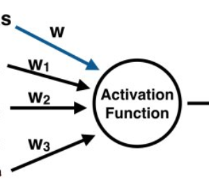
An ANN is a design defined by an activation function, which is practised by interconnected information processing assemblies to reconstruct input into output. Artificial Neural Network has always been compared to the human brain. The first layer of the neural network acquires the raw input, treats it and transfers the prepared information to the hidden layers. The hidden layer transfers the information to the last layer, which generates the output. The choice of an ANN is that it is adaptive in nature. It reads from the information provided which means that it trains itself from the data, which has a perceived outcome and optimises its weights for a better prophecy in situations with an unknown outcome.
A perceptron, which is a single layer neural network, is the most elementary form of a neural network. The perceptron supports multidimensional input and prepares it utilising a weighted summation and an activation purpose. It is trained using a labelled data and learning algorithm that optimise the weights in the summation processor. A significant limitation of the perceptron model is its inability to deal with non-linearity. A multilayered neural network succeeds in this limitation and assists solve non-linear problems. The input layer connects with a hidden layer, which in turn connects to the output layer. The connections are weighted and weights are optimized for applying a learning rule.
Fitting Neural Network in R
The neural network fitting in R starts with data fitting into ANN
Data Fitting
Data fitting is the method of building a circuit or a mathematical function that has the
best approximation with a set of previously collected points. The circuit fitting can be compared with both interpolations, where accurate data points are required, and smoothing, where a flat
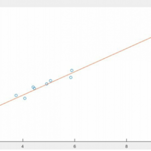
function is built that approximates the data. The estimated curves collected from the data fitting can be used to help display data, to predict the values of a function where no data is available, and to summarise the relationship between two or more variables.
Input-Output Relationship
Once the neural network is provided with the data, it forms a generalisation of the input-output relationship and can be applied to produce outputs for inputs it was not modelled on.
In this example, we will consider the fuel consumption of vehicles which has always been studied by the major manufacturers of the automobile industry.
In an era designated by oil refuelling dilemmas and even prominent air pollution problems, fuel consumption by vehicles has become a key factor. In this example, we will build a neural network with the purpose of predicting the fuel consumption of vehicles depending on certain characteristics.
The dataset contains gas mileage, horsepower, and other information of some vehicles. It is a data frame has the following nine variables:
- mp_g: Miles per gallon.
- cylinders_48: Number of cylinders between 4 and 8.
- dis_placement: Engine displacement (cubic inches).
- horse_power: Engine horsepower.
- weight_lbs: Vehicle weight (lbs).
- acceleration_mph: Time to accelerate from 0 to 60 mph (sec).
- year_r: Model year (modulo 100).
- origin_c: Origin of the car (American, European, Japanese).
- name_v: Vehicle name.
R Code
library("neuralnet")

library("ISLR") // for obtaining auto dataset//

data = Auto

View(data)

plot(data$weight_lbs, data$mp_g, pch=data$origin_c,cex=2)

par(mfrow=c(2,2))

plot(data$cylinders_48, data$mp_g, pch=data$origin_c,cex=1)

plot(data$dis_placement, data$mp_g, pch=data$origin_c,cex=1)

plot(data$horse_power, data$mp_g, pch=data$origin_c,cex=1)

plot(data$acceleration_mph, data$mp_g, pch=data$origin_c,cex=1)

mean_data <- apply(data[1:6], 2, mean)

sd_data <- apply(data[1:6], 2, sd)

data_scaled <- as.data.frame(scale(data[,1:6],center = mean_data, scale = sd_data))

head(data_scaled, n=20)

index = sample(1:nrow(data),round(0.70*nrow(data)))

train_data <- as.data.frame(data_scaled[index,])

test_data <- as.data.frame(data_scaled[-index,])

n = names_v(data_scaled)

f = as.formula(paste("mpg ~", paste(n[!n %in% "mpg"], collapse = " + ")))

net = neuralnet(f,data=train_data,hidden=3,linear.output=TRUE)

plot(net)

predict_net_test <- compute(net,test_data[,2:6])

MSE.net <- sum((test_data$mpg - predict_net_test$net.result)^2)/nrow(test_data)

Lm_Mod <- lm(mpg~., data=train_data)

summary(Lm_Mod)

predict_lm <- predict(Lm_Mod,test_data)

MSE.lm <- sum((predict_lm - test_data$mpg)^2)/nrow(test_data)

Lm_Mod <- lm(mpg~., data=train_data)

summary(Lm_Mod)

predict_lm <- predict(Lm_Mod,test_data)

MSE.lm <- sum((predict_lm - test_data$mpg)^2)/nrow(test_data)

par(mfrow=c(1,2))

plot(test_data$mp_g,predict_net_test$net.result,col='black',main='Real vs predicted for neural network',pch=18,cex=4)construction

abline(0,1,lwd=5)

plot(test_data$mpg,predict_lm,col='black',main='Real vs predicted for linear regression',pch=18,cex=4)

abline(0,1,lwd=5)
The ISLR library command loads the auto dataset, which, as anticipated, is contained in the ISLR library, and saves it in a given data frame. Using the View function to view a compressed display of the structure of an arbitrary R object.
Exploratory analysis
We carry out an exploratory analysis to know how data is distributed and obtain preliminary knowledge. The process begins by explorative analysis by tracing a plot of predictors versus objective. The predictors are the following variables: cylinders, displacement, horsepower, weight, acceleration, year, origin, and name. The target is the mp_g variable that contains measurements of the miles per gallon sample cars.
The following are the other graphs, that plot the remaining numeric predictors (cylinders, displacement, horsepower, and acceleration) versus target (mpg).
R Code
par(mfrow=c(2,2))

plot(data$cylinders_48, data$mp_g, pch=data$origin_c,cex=1)

plot(data$dis_placement, data$mp_g, pch=data$origin_c,cex=1)

plot(data$horse_power, data$mp_g, pch=data$origin_c,cex=1)

plot(data$acceleration_mph, data$mp_g, pch=data$origin_c,cex=1)(/code)
Building A Neural Network Model
It is recommended to normalise the data before exercising a neural network. With normalisation, data units are reduced, allowing users to easily associate data from various locations. It is not that the data is always needed to be normalized numeric data. Nevertheless, it has been noticed that when numeric values are normalized, neural network formation is often more practical and leads to better prediction.
In fact, if numeric data are not normalised and the sizes of two predictors are very inaccessible, a change in the value of a neural network weight has a much more relevant influence on the higher value. There are several standardisation techniques out of which min-max standardization and Z-scored normalisation are preferred due to there simplicity and. The Z-scored technique consists of deducting the mean of the column to each value in a column and then distributing the result for the standard deviation of the column.
Building A Neural Network Model
It is recommended to normalise the data before exercising a neural network. With normalisation, data units are reduced, allowing users to easily associate data from various locations. It is not that the data is always needed to be normalized numeric data. Nevertheless, it has been noticed that when numeric values are normalized, neural network formation is often more practical and leads to better prediction. In fact, if numeric data are not normalised and the sizes of two predictors are very inaccessible, a change in the value of a neural network weight has a much more relevant influence on the higher value.
There are several standardisation techniques out of which min-max standardization and Z-scored normalisation are preferred due to there simplicity and. The Z-scored technique consists of deducting the mean of the column to each value in a column and then distributing the result for the standard deviation of the column.
Once the data is normalised everything is set to construct a Neural Network. While constructing the Neural Network the following points are to be considered.
- A small number of neurons will drive to a high error for the systems, as the predictive portions might be too complicated for a small number of neurons to capture
- A large number of neurons will overfit the training data and not induce well
- The number of neurons in each hidden layer should be about the size of the input and the output layer, probably the mean
- The number of neurons in each hidden layer shouldn’t surpass twice the number
of input neurons, as you are probably grossly overfitting at a given point
In this illustration, we have five input variables (cylinders, displacement, horsepower, weight, and acceleration) and one variable output (mpg). Let three neurons be in the hidden layer.
net_# = neuralnet(f,data=train_data,hidden=3,linear.output=TRUE)
The hidden argument allows a vector with the number of neurons for each hidden layer, while the argument linear.output is applied to specify whether we want to do regression(linear.output=TRUE) or classification (linear.output=FALSE).
The three main features of the neural network component are listed below:
Length: This is component length, which showcases how many elements of this type are contained in it
Class: contains particular indication on the component class
Mode: A type of component.


