A beginner’s guide to Chi-square test in python from scratch

Consider that you are exploring a dataset, and you are wondering if there is a relationship between the two categorical variables? To check this, you can go through an effective statistical test and in this scenario, the Chi-square test is the most suitable one. The Chi-square test is one of the statistical tests we can use to decide whether there is a correlation between the categorical variables by analysing the relationship between the observed and expected values. In this article, we will discuss the Chi-square test and we will understand its implementation in Python from scratch by taking random data. The major points to be discussed in this article are listed below. 

Table of contents

1. What is chi-square?
2. Where chi-square is used?
3. Introduction to data
4. Implement chi-square
5. Yate’s Correction

Let’s begin with understanding what Chi-square test is.

What is Chi-square?

The Chi-square test is a statistical test used to determine the relationship between the categorical variables/columns in the dataset. It examines the correlation between the variables which do not contain the continuous data.

How to use the Chi-square test?

To use the chi-square test, we can take the following steps:

1. Define the null (H0) and alternative (H1) hypothesis.
2. Determine the value of alpha (𝞪) for according to the domain you are working. Ideally 𝞪=0.05 that means you are willing to take 0.5% of risk/ margin of error.
3. Check the data for Nans or other kind of errors.
4. Check the assumptions for the test.
5. At last perform the test and draw your conclusion  whether to reject or support null hypothesis (H0) .   

The formula for the Chi-square test is given as:-

Where, 

= chi-square

= observed value

= expected value

The Chi-square formula is a statistical method to compare two or more data samples. It is used with data that consist of variables distributed across various categories and is denoted by .

Where is the Chi-square test used?

Pearson’s chi-squared test is a hypothesis test that is used to determine whether there is a significant association between two categorical variables in the data. The test involves two hypotheses (H0 & H1):

• H0 : The two categorical variables have no relationship (independent)
• H1 : There is a relationship (dependent) between two categorical variables

So as a null hypothesis, we keep the positive aspect of the test and in the alternate hypothesis, we keep the negative aspect. The positive aspect of chi-square is that there should not be any correlation because correlation can result in overfitting of the machine learning algorithm. The negative is that there is a correlation between the two categorical columns.

In the next section of the article, I would introduce you to the data on which we are going to implement the chi-square test to see whether they are co-related.

Introduction to data

We will create a random table for implementing the Chi-square test and check whether there is a relation between the columns. We will follow these steps to create a contingency table:

Step 1: Importing libraries to create an array and data frame:

import numpy as np

import pandas as pd

Step 2: Creating an array and converting that array to the data frame:

np.random.seed(10)
# Sample data randomly at fixed probabilities
type_bottle = np.random.choice(a= ["paper","cans","glass","others","plastic"],
                              p = [0.05, 0.15 ,0.25, 0.05, 0.5],
                              size=1000)
 
# Sample data randomly at fixed probabilities
month = np.random.choice(a= ["January","February","March"],
                              p = [0.4, 0.2, 0.4],
                              size=1000)
 
bottles = pd.DataFrame({"types":type_bottle, 
                       "months":month})
 
bottles_tab = pd.crosstab(bottles.types, bottles.months, margins = True)
 
bottles_tab.columns = ["January","February","March","row_totals"]
 
bottles_tab.index = ["paper","cans","glass","others","plastic","col_totals"]
 
observed = bottles_tab.iloc[0:5,0:3]   # Get table without totals for later use
bottles_tab

After executing the above lines of codes, the output would look like this:

The above contingency table shows the different types of bottles (category) as an index that have been recycled in the month of January, February, March. Row_total and column_total show the total sum of each category (type of bottles) and month total collection respectively.

Implementing the Chi-square test

Let’s implement the Chi-square test and check the independence of columns. So in the formula discussed above, we need two things: observed values and expected values. So we need to understand how to calculate these values. The observed value is nothing but the original data.

How to calculate expected values?

Multiply the row total to the column total and divide by the total number of observations for a cell to get the expected count. So, to calculate the expected counts in python we need to use the np.outer() function on row total and column total. At last, dividing the output of the np.outer() function by observations.

Now, as explained, let us code the above explanation in python.

expected =  np.outer(bottles_tab["row_totals"][0:5],
                     bottles_tab.loc["col_totals"][0:3]) / 1000
 
expected = pd.DataFrame(expected)
 
expected.columns = ["Janurary","Feburary","March"]
expected.index = ["paper","cans","glass","others","plastic"]
 
expected

Here, we will write the formula in python to calculate the chi-square static value.

chi_squared_stat = (((observed-expected)**2)/expected).sum().sum()

print(chi_squared_stat)

Note: We call .sum() twice, once to get the column sums and a second time to add the column sums together, returning the sum of the entire 2D table.

Next, we will calculate the p-value and critical value which will help to accept or reject the null hypothesis.

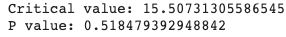
critical_value= chi2.ppf(q = 0.95, # Find the critical value for 95% confidence*
                      df = 8)   # df= degree of freedom
 
print("Critical value:",critical_value)
 
p_value = 1 - chi2.cdf(x=chi_squared_stat,  # Find the p-value
                             df=8)
print("P value:",p_value)

Note: The degrees of freedom for a test of independence equals the product of the number of categories in each variable minus 1. In this case we have a 5×3 table so df = 4×2 = 8.

In the above explanations, we have seen how does chi-square test work. It can be done by a quick method by just a single line of code, which is given below, without doing all of the above steps: 

scipy.stats.chi2_contingency(observed= observed)

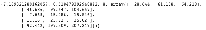
Finally, we get a p-value of 0.51847 which is greater than 0.5. Therefore, we will accept the null hypothesis that says there is no relationship between the features. The test result does not detect a significant relationship between the variables.

Yate’s Correction

In the above explanation of the Pearson’s chi-square formula that was a fault which was corrected by Frank Yates, and it’s known as Yate’s correction or Yate’s Chi-Square. Yate’s Chi-square formula is given as:

O_i = an observed frequency

E_i = an expected (theoretical) frequency

N = number of distinct events

Yate corrected Pearson’s chi-square formula by subtracting the difference of the observed and expected value by 0.5 and the rest is the same as the previous.

To use Yate’s chi-square test, we can write the following line of code: 

scipy.stats.chi2_contingency(df, correction=True)  #"correction=True" to apply Yates' correction           

Conclusion

To analyze the relationship between variables in the dataset, we conducted a Chi-square test for independence in this article. We used SciPy and started with data from scratch. We could learn how to implement this test practically and how to make inferences about the data.

Hope you have enjoyed reading this article :) 

References

1. Link for the above codes
2. Scipy Documentation