Last updated March 12, 2021
In AI Mysteries

A Beginners Guide To Regression Techniques

Share

Published on January 13, 2020

by Rohit Garg

Regression analysis is a form of predictive modelling technique which investigates the relationship between a dependent (target) and independent variable (s) (predictor). This technique is used for finding the relationship between the variables.

Example: Let’s say, you want to estimate growth in sales of a company based on current economic conditions. You have the recent company data which indicates that the growth in sales is around two and a half times the growth in the economy. Using this insight, we can predict future sales of the company based on current & past information.

It indicates the significant relationships between the dependent variable and independent variable. It indicates the strength of the impact of multiple independent variables on a dependent variable

Content

1. Terminologies related to regression analysis
2. Linear regression
3. Logistic regression
4. Bias – Variance
5. Regularization
6. Performance metrics – Linear Regression
7. Performance metrics – Logistic Regression

Outliers: Suppose there is an observation in the dataset which is having very high or very low value as compared to the other observations in the data, i.e. it does not belong to the population, such an observation is called an outlier. In simple words, it is an extreme value. An outlier is a problem because many times it hampers the results we get.

Multicollinearity: When the independent variables are highly correlated to each other than the variables are said to be multicollinear. Many types of regression techniques assume multicollinearity should not be present in the dataset. It is because it causes problems in ranking variables based on its importance. Or it makes the job difficult in selecting the most important independent variable (factor).

Heteroscedasticity: When the dependent variable’s variability is not equal across values of an independent variable, it is called heteroscedasticity. Example – As one’s income increases; the variability of food consumption will increase. A poorer person will spend a rather constant amount by always eating inexpensive food; a wealthier person may occasionally buy inexpensive food and at other times eat expensive meals. Those with higher incomes display a greater variability of food consumption.

Underfitting and Overfitting: When we use unnecessary explanatory variables, it might lead to overfitting. Overfitting means that our algorithm works well on the training set but is unable to perform better on the test sets. It is also known as the problem of high variance. When our algorithm works so poorly that it is unable to fit even training set well then it is said to underfit the data. It is also known as the problem of high bias.

Autocorrelation: It states that the errors associated with one observation are not correlated with the errors of any other observation. It is a problem when you use time-series data.

Suppose you have collected data from type of food consumption in eight different states. It is likely that the food consumption trend within each state will tend to be more like one another that consumption from different states i.e. their errors are not independent.

2. Linear Regression

Suppose you want to predict the amount of ice cream sales you would make based on the temperature of the day, then you can plot a regression line that passes through all data points.

Least squares are one of the methods to find the best fit line for a dataset using linear regression. The most common application is to create a straight line that minimizes the sum of squares of the errors generated from the differences in the observed value and the value anticipated from the model. Least-squares problems fall into two categories: linear and nonlinear squares, depending on whether the residuals are linear in all unknowns.

2.1. Important assumptions in regression analysis:

There should be a linear and additive relationship between the dependent (response) variable and the independent (predictor) variable(s). A linear relationship suggests that a change in response Y due to one unit change in X is constant, regardless of the value of X. An additive relationship suggests that the effect of X on Y is independent of other variables.

There should be no correlation between the residual (error) terms. Absence of this phenomenon is known as Autocorrelation.

The independent variables should not be correlated. Absence of this phenomenon is known as multicollinearity.

The error terms must have constant variance. This phenomenon is known as homoskedasticity. The presence of non-constant variance is referred to as heteroskedasticity.

The error terms must be normally distributed.

3. Logistic Regression

Logistic regression is based on Maximum Likelihood (ML) Estimation which says coefficients should be chosen in such a way that it maximizes the probability of Y given X (likelihood). With ML, the computer uses different “iterations” in which it tries different solutions until it gets the maximum likelihood estimates.

Fisher Scoring is the most popular iterative method of estimating the regression parameters.

logit(p) = b0 + b1X1 + b2X2 + —— + bk Xk

where logit(p) = ln(p / (1-p))

p: the probability of the dependent variable equaling a “success” or “event”.

The reason for not using linear regression for such cases is that the homoscedasticity assumption is violated. Errors are not normally distributed. Y follows a binomial distribution.

3.1. Interpretation of Logistic Regression Estimates:

If X increases by one unit, the log-odds of Y increases by k unit, given the other variables in the model are held constant.

In logistic regression, the odds ratio is easier to interpret. That is also called Point estimate. It is the exponential value of the estimate.

For Continuous Predictor: An unit increase in years of experience increases the odds of getting a job by a multiplicative factor of 4.27, given the other variables in the model are held constant.

For Binary Predictor: The odds of a person having years of experience getting a job are 4.27 times greater than the odds of a person having no experience.

3.2. Assumptions of Logistic Regression:

The logit transformation of the outcome variable has a linear relationship with the predictor variables.

The one way to check the assumption is to categorize the independent variables. Transform the numeric variables to 10/20 groups and then check whether they have a linear or monotonic relationship.

No multicollinearity problem.

No influential observations (Outliers).

Large Sample Size – It requires at least 10 events per independent variable.

3.3. Odd’s ratio

In logistic regression, odds ratios compare the odds of each level of a categorical response variable. The ratios quantify how each predictor affects the probabilities of each response level.

For example, suppose that you want to determine whether age and gender affect whether a customer chooses an electric car. Suppose the logistic regression procedure declares both predictors to be significant. If GENDER has an odds ratio of 2.0, the odds of a woman buying an electric car are twice the odds of a man. If AGE has an odds ratio of 1.05, then the odds that a customer buys a hybrid car increase by 5% for each additional year of age

Odd Ratio (exp of estimate) less than 1 ==> Negative relationship (It means negative coefficient value of estimate coefficients)

4. Bias – Variance

Error due to Bias: It is taken as the difference between the expected prediction of the model and the actual value. Bias measures how far off, in general, the predictions are from the actuals.

Error due to Variance: It is taken as the variability of a model prediction for a given data pint. The variance is how much the prediction varies for different models.

4.1. Interpretation of Bias – Variance

Imagine that the center of the target is a model that perfectly predicts the correct values. As we move away from the bulls-eye, our predictions get worse and worse.
Imagine we can repeat our entire model building process to get several separate hits on the target.
Each hit represents an individual realization of our model, given the chance variability in the training data we gather.

4.2. Bias – Variance Trade-Off

Bias is reduced and variance is increased in relation to model complexity.
As more and more parameters are added to a model, the complexity of the model rises, and variance becomes our primary concern while bias steadily falls.

5. Regularization

Regularization helps to solve over fitting problem which implies model performing well on training data but performing poorly on validation (test) data. Regularization solves this problem by adding a penalty term to the objective function and control the model complexity using that penalty term. We do not regularize the intercept term. The constraint is just on the sum of squares of regression coefficients of X’s.

Regularization is generally useful in the following situations:

Large number of variables
Low ratio of number observations to number of variables
High Multi-Collinearity

L1 Regularization:

In L1 regularization we try to minimize the objective function by adding a penalty term to the sum of the absolute values of coefficients.
This is also known as least absolute deviations method.
Lasso Regression makes use of L1 regularization.

L2 Regularization:

In L2 regularization we try to minimize the objective function by adding a penalty term to the sum of the squares of coefficients.
Ridge Regression or shrinkage regression makes use of L2 regularization.

5.1. Lasso Regression

Lasso (Least Absolute Shrinkage and Selection Operator) penalizes the absolute size of the regression coefficients. Lasso regression used L1 regularization. In addition, it can reduce the variability and improving the accuracy of linear regression models.

Lasso regression differs from ridge regression in a way that it uses absolute values in the penalty function, instead of squares. This leads to penalizing (or equivalently constraining the sum of the absolute values of the estimates) values which causes some of the parameter estimates to turn out exactly zero. Larger the penalty applied, further the estimates get shrunk towards absolute zero. This results in variable selection out of given n variables.

5.2. Ridge Regression

Ridge Regression is a technique used when the data suffers from multicollinearity. Ridge regression uses L2 regularization. In multicollinearity, even though the least squares estimate (OLS) are unbiased, their variances are large which deviates the observed value far from the true value. By adding a degree of bias to the regression estimates, ridge regression reduces the standard errors.

In a linear equation, prediction errors can be decomposed into two sub components. First is due to the bias and second is due to the variance. Prediction error can occur due to any one of these two or both components. Here, we’ll discuss the error caused due to variance. Ridge regression solves the multicollinearity problem through Shrinkage Parameter λ (lambda).

6. Performance Metrics – Linear Regression Model

6.1. R-Squared

It measures the proportion of the variation in your dependent variable explained by all your independent variables in the model.
Higher the R-squared, the better the model fits your data.

SS-res denotes residual sum of squares

SS-tot denotes total sum of squares

6.2. Adjusted R-Square

The use of adjusted R2 is an attempt to take account of non-explanatory variables that are added to the model. Unlike R2, the adjusted R2 increases only when the increase in R2 is due to significant independent variable that affects dependent variable
The adjusted R2 can be negative, and its value will always be less than or equal to that of R2.

k denotes the total number of explanatory variables in the model

n denotes the sample size.

6.3. Root Mean Square Error (RMSE)

It explains how close the actual data points are to the model’s predicted values.
It measures standard deviation of the residuals.

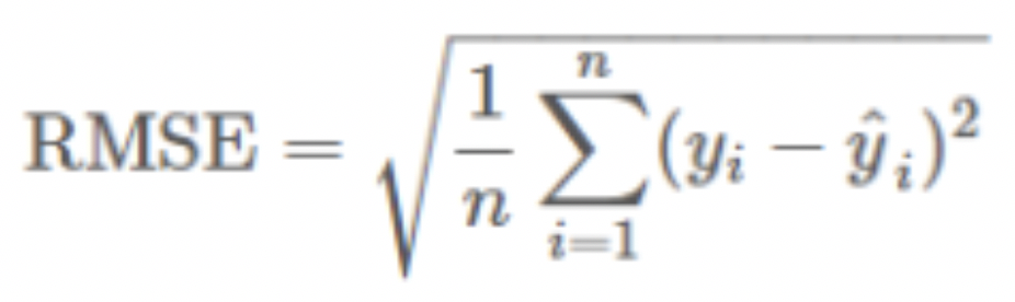
yi denotes the actual values of dependent variable

yi-hat denotes the predicted values

n – denotes sample size

6.4. Mean Absolute Error (MAE)

MAE measures the average magnitude of the errors in a set of predictions, without considering their direction.
It’s the average over the test sample of the absolute differences between prediction and actual observation where all individual differences have equal weight.

7. Performance Metrics – Logistic Model

7.1. Performance Analysis (Development Vs OOT)

The Kolmogorov-Smirnov (KS) test is used to measure the difference between two probability distributions.
For example, the distribution of the good accounts and the distribution of the bad accounts with the score.

7.2. Model Alignment

Model alignment is done by calculating the PDO (Point of Double Odds). The objective of scaling is to convert the raw (model output) score into a scaled score so that Business can assess and track changes in risk effectively.
The PDO is calculated only on the good and the bad observations. For a scale to be specified, the following three measurements need to be provided.

1. Reference score: This can be any arbitrary score value, taken as a reference point.
2. Odds at reference score: The odds of becoming a bad, at the reference score.
3. PDO: Points to Double odds.

7.3. Model Accuracy

Model accuracy is checked by calculating the Bad Count error percentage (BCEP) for Development and OOT sample.
Check whether the BCEP for each model was within the permissible limit of +/- 25%

7.4. Model Stability

To confirm whether the model is stable over time, we check the Population stability Index (PSI) in Development and OOT sample.
Check whether the PSI is within the range of +/- 25%

Access all our open Survey & Awards Nomination forms in one place

Rohit Garg

Rohit Garg has close to 7 years of work experience in field of data analytics and machine learning. He has worked extensively in the areas of predictive modeling, time series analysis and segmentation techniques. Rohit holds BE from BITS Pilani and PGDM from IIM Raipur.