When it comes to determining whether a business will succeed or fail, time is the most important factor. Pre-processing, trend normalization, and, most importantly, a cross-check of all available algorithms take time when building a robust forecasting model from scratch. There are a variety of AutoML tools in the market that allow us to perform modelling on raw data with just a few lines of code, saving our time. However, in this article, we will concentrate on PyCaret, an AutoML tool. Time series modelling necessitates special treatment due to the presence of its component, which PyCaret provides. The main points to be discussed in this article are given in the below table of contents.
Table of Contents
- What is Time Series Modelling?
- All About PyCaret
- Quick Start Modelling with PyCaret
Let’s start the discussion by understanding what time series modelling is.
What is Time Series Modelling
A time series is a quantity that is measured over time in a progressive manner. In its broadest sense, time series analysis attempts to forecast what will happen in the future by inferring what happened to a set of data points in the past. We will, however, approach time series quantitatively by assuming that they are realizations of random variable sequences.
To put it another way, we will assume that our time series are generated by an underlying generating process based on one or more statistical distributions from which these variables are drawn. The goal of time series analysis is to learn about the past while also predicting the future.
Time series data is naturally organized chronologically. Time series analysis differs from cross-sectional research in which the observations are not naturally ordered (for example, explaining people’s earnings by reference to their educational degrees, where the individuals’ data might be input in any order).
Time series analysis varies from spatial data analysis in that the observations are typically linked to specific physical places (e.g. accounting for house prices by the location as well as the intrinsic characteristics of the houses).
In general, a stochastic model for a time series will represent the fact that observations near in time are more tightly related than ones further away. Furthermore, time series models commonly use the inherent one-way ordering of time to express values for a given period as derived from past rather than future values.
All About PyCaret
PyCaret is a low-code machine learning library and end-to-end model management solution for automating machine learning workflows that are created in Python. It is quite popular due to its ease of use, simplicity, and ability to quickly and efficiently construct and deploy end-to-end machine learning prototypes.
PyCaret is a low-code alternative that may be used to replace hundreds of lines of code with just a few lines. As a result, the experiment cycle becomes exponentially faster and more efficient.
PyCaret is a straightforward and straightforward application. All of PyCaret’s operations are saved in a Pipeline, which is fully automated and ready for deployment. PyCaret automates everything from missing values through one-hot encoding, categorical data transformation, feature engineering, and hyperparameter tuning.
Quick Start With PyCaret
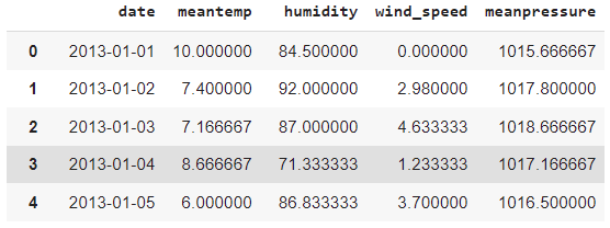
In this section, we will leverage the power of PyCaret to model Time Series Data. The dataset used is of climate parameters such as temperature, humidity, wind pressure, and an atmospheric pressure of a city in Delhi. All the instances are recorded from the year 2013 to 2017 and it is taken from this Kaggle repository.
To work with PyCaret you need to install it via simply pip command like! pip install pycaret[full] which installs all the core functionality of the package. Now let’s take a look at the dataset.
import pandas as pd
data = pd.read_csv('/content/DailyDelhiClimateTrain (2).csv')
data
As you know, the time series forecasting or modelling is a kind of regression model for that we can use PyCaret’s regression module to deal with it.
The PyCaret Regression Module is a supervised machine learning module that computes the relationships between one or more independent variables and one or more dependent variables (also known as the “outcome variable”, or “target”). Regression is used to anticipate continuous data such as sales amount, quantity, temperature, and customer count. The setup function in PyCaret provides a number of pre-processing options for preparing data for modelling across all modules.
The default settings of PyCaret’s Regression module are not ideal for time series data because they involve a few data preparation steps that are not valid for ordered data (data with a sequence such as time series data).
Time-series data necessitates a different type of cross-validation because the order of dates must be preserved. When evaluating models, the PyCaret regression module employs k-fold random cross-validation by default. For time-series data, the default cross-validation setting is insufficient. Because algorithms cannot deal with dates directly, we have extracted some simple features from dates, such as month and year, and removed the original date column.
Now here we are using only one feature from our data because, at the time of predicting the values of the features, we also need to supply close realistic values for those independent variables which are hard to simulate the same as data we have. But we can also extend it to multiple features prediction as usual by holding a test split from data but make sure you do not shuffle the data as it is a time series problem.
data['month'] = [i.month for i in data['date']]
data['year'] = [i.year for i in data['date']]
data['day_of_week'] = [i.dayofweek for i in data['date']]
data['day_of_year'] = [i.dayofyear for i in data['date']]
Let’s split data for train and test.
train = data[data['year'] < 2016]
test = data[data['year'] >= 2016]
Now we will explicitly pass the training data, test data, and cross-validation strategy to the setup function via the fold strategy parameter.
from pycaret.regression import *
# initialize setup
Setup_ = setup(data = train, test_data = test, target = ['meantemp'], fold_strategy = 'timeseries', numeric_features = ['year','month','day_of_week','day_of_year'], fold = 3, transform_target = True, session_id = 123)
Now let’s train and validate all the available models:
best = compare_models(sort = 'MAE')
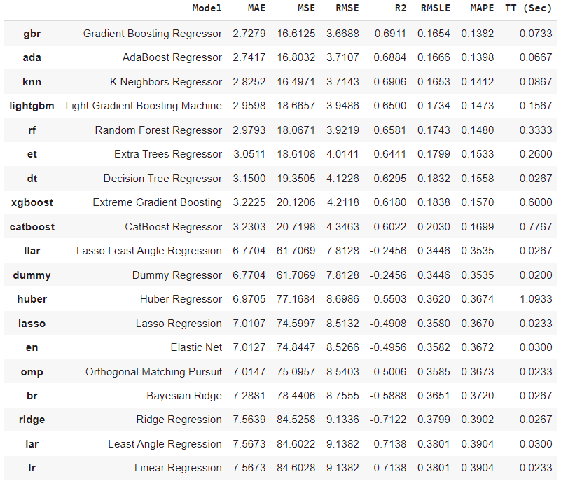
PyCaret does provide a detailed report of all the models, same as other AutoML tools. We have sorted the result based on Mean Absolute Error and based on that Gradient Booster regressor outperforms the rest not only w.r.to MAE but also with all other metrics.
Technically speaking, we have trained these models on only features and those retrieved from simple date format. In order to make a future prediction, we need to simulate the same four attributes from the date format.
As you have seen, the last observation of our data is on 2017-01-01, now we are going to create some future instances up to 2019-01-01 nearly for 2 years. We are expecting that the model should predict the same trend as it has seen previously.
future_dates = pd.date_range(start = '2017-01-02', end = '2019-01-01', freq = 'D')
future_df = pd.DataFrame()
future_df['month'] = [i.month for i in future_dates]
future_df['year'] = [i.year for i in future_dates]
future_df['day_of_week'] = [i.dayofweek for i in future_dates]
future_df['day_of_year'] = [i.dayofyear for i in future_dates]
Now let’s finalize the model and make the predictions.
final_best = finalize_model(best)
predictions_future = predict_model(final_best, data=future_df)
Now we will visualize the result using Plotly express. Plotly is an open-source library used widely to create beautiful and more insightful visualization. To know more about the Plotly visualization, you can refer to this article.
concat_df = pd.concat([data,predictions_future], axis=0)
concat_df_i = pd.date_range(start='2013-01-01', end = '2019-01-01', freq = 'D')
concat_df.set_index(concat_df_i, inplace=True)
fig = px.line(concat_df, x=concat_df.index, y=["meantemp", "Label"])
fig.show()

What do you think by observing the above result? I would say it is the more beautiful plot I have ever seen. Because the models have mostly identified major trends in data especially the peak trend and downtrend.
Conclusion
Technically we have done the univariate modelling, but it resembles multivariate because we have used four features like day, month, year, and day of the year. As we discussed earlier, for multivariate modelling, we can pass multiple features inside the setup function for the attribute numeric_features.
Through this post, we have discussed what time series modelling is, and in contrast to a low code base, we practically see how an AutoML tool like PyCaret can be used to perform outstanding modelling.


