A Complete Guide to Causal Inference in Python

In data analytics and machine learning, when we apply the behavioural science insights in the studies, it always helps in improving the experience in delivering the results. One of the most important areas of behavioural science is the causal inference which is basically used for extracting cause and intensity of cause. It belongs to the family of loosely connected methods. In this article, we will have a detailed discussion of causal inference and we will try to understand its importance with hands-on implementations. The major points to be covered in the article are listed below.

Table of Contents 

1. What is Causal Inference?
2. Why is Causal Inference Important?
3. Varieties of Causal Inference 
4. Causal Inference in Python
   1. Data Preparation and Mathematical Analysis
   2. Goals
   3. Making Assumption
5. Modelling the Counterfactual
6. Covariate Imbalance
7. Propensity Score
8. Unconfoundedness and the Propensity Score
   1. Trimming
   2. Stratification

What is Causal Inference?

In statistics, there is always a question that comes to the mind of researchers that “why is something happening?”  Here the point which comes into focus is the causal inference which can be considered as the family of statistical methods whose main motive is to give the reasons for any happening. We use causal inference to determine the cause of changes in one variable if the changes occur in a different variable where standard statistical approaches like regression are being used to determine how the changes in one variable are associated with the changes in another variable. 

Let’s suppose there are two variables X and Y. The standard methods here will focus on determining the association whereas the causal inference approaches will be concerned about why the variable X changes if it is causally related with the variable Y so that we can explain changes in X in terms of changes in the Y variable.

Why is Causal Inference Important?

At every level of statistics, causal inference is used for providing a better user experience for customers on any platform. We can use the insights of causal inferences to identify the problems related to the customer or problems occurring in the organization. Also, it can be used to improve the customer experience. For example, any product introducing a new feature and the customers are raising complaints about the new feature due to lack of clarity or he is confused about the procedure of using the new feature. In such a scenario we can improve the communication about the usage or procedure of usage of a new feature instead of giving news updates on it or dropping down the new feature plans.

Causal inference can be used to make information that can help in improving the user experience and also we can generate business decisions by knowing its impact on the business.

If we can understand the relationship between two intangible variables such as employee satisfaction and business metrics, we will be able to use such information to prioritize tasks and aim for new features and tools. Also, these inferences can help in understanding the short-term and long-term impact of any new decision or program.

Causal inference enables us to answer questions that are causal based on observational data, especially in situations where testing is not possible or feasible. For example, we started a campaign where users of our product can participate and mail their queries and complaints and we want to measure the impact of the campaign on the business. Causal inference enables us to find answers to these types of questions which can also lead to better user experiences on any platform.

Varieties of Causal Inference

Since causal inference is a combination of various methods connected together, it can be categorized into various categories for a better understanding of any beginner. We can say there can be two categories according to the data. These two categories are :

• Causal inference with experimental data
• Causal inference with observational data

Causal Inference in Python

In this article, we are going to make causal inferences using observational data and also we will use a package named CausualInference for performing our analysis.

Let’s start with an example where a supervisor notices that from his team of several labourers, labourers who are properly dressed up according to the norms tend to be less productive than the labourers who are not properly dressed up. The supervisor starts with making the data about the labourers where he puts value 1 for those who are dressed up and 0 for those who are in casual dresses and the productive section he puts 1 if the labourer is productive otherwise he puts 0. He makes the data for a whole week.

Data Preparation and Mathematical Analysis

Let’s make this type of data using python:

import numpy as np
import pandas as pd
p_z = 0.5
p_x_z = [0.9, 0.1]
p_y_xz = [0.2, 0.4, 0.6, 0.8]
z = np.random.binomial(n=1, p=p_z, size=500)
p_x = np.choose(z, p_x_z)
x = np.random.binomial(n=1, p=p_x, size=500)
p_y = np.choose(x+2*z, p_y_xz)
y = np.random.binomial(n=1, p=p_y, size=500)
generate_dataset_0 = pd.DataFrame({"x":x, "y":y})
generate_dataset_0

Output:

Here in the data, we have 500 samples of labourers. Where X is about their dressing and Y is about the productiveness of labourers.

The first question in casualty which comes to mind is what is the quantity of labourers who are dressed up but not productive. 

We can simply calculate it by:

P(Y=1|X=1)−P(Y=1|X=0)

Where p is probability and we can estimate the quantity in python using the following function.

def estimate_uplift(ds):
    base = ds[ds.x == 0]
    variant = ds[ds.x == 1]
    delta = variant.y.mean() - base.y.mean()
    delta_err = 1.96 * np.sqrt(
        variant.y.var() / variant.shape[0] + 
        base.y.var() / base.shape[0])
    return {"estimated_effect": delta, "standard_error": delta_err}
estimate_uplift(generate_dataset_0)

Output:

Here from this, we can infer that labourers who are dressed up are less productive. Using the above code we have estimated the means of two groups.

Here the “estimated_effect” – the difference in mean values of y for productive and unproductive samples and  “standard_error” – 90% confidence intervals around “estimated_effect”.

To be more sure about the estimation we can run the chi-square contingency test.

from scipy.stats import chi2_contingency
contingency_table = (
    generate_dataset_0
    .assign(placeholder=1)
    .pivot_table(index="x", columns="y", values="placeholder", aggfunc="sum")
    .values
)
_, p, _, _ = chi2_contingency(contingency_table, lambda_="log-likelihood")
# p-value
p

Output:

That’s a small p-value.

Using the above-generated information we can estimate any labourer’s probability if we see them dressed up. But we need to believe that the observations are drawn from the same distribution.

Till now we are using randomly generated small data for the analysis and according to that, we can suggest the supervisor use this information to decide whether the labourer should be dressed up or not. If the supervisor does this he fundamentally changes the system in which we are making inferences, this can alter or reverse the correlation that we observed.

We can measure the changes in the system by randomized controlled trials, which is randomizing the observation about who is dressed up and who isn’t, and looking for different values in the productive section. Using this we can remove the effect of any confounding variables which can cause changes in the metric we care about.

Let’s draw a function to generate the dataset so that we can intervene in the function directly and go on with the procedure of the A/B test.

import numpy as np
import pandas as pd
from sklearn.preprocessing import PolynomialFeatures
def generate_dataset_0(n_samples=500, set_X=None, show_z=False):
    p_z = 0.5
    p_x_z = [0.9, 0.1]
    p_y_xz = [0.2, 0.4, 0.6, 0.8]
    z = np.random.binomial(n=1, p=p_z, size=n_samples)
    if set_X is not None:
        assert(len(set_X) == n_samples)
        x = set_x
    else:
        p_x = np.choose(z, p_x_z)
        x = np.random.binomial(n=1, p=p_x, size=n_samples)
    p_y = np.choose(x+2*z, p_y_xz)
    y = np.random.binomial(n=1, p=p_y, size=n_samples)
    if show_z:
        return pd.DataFrame({"x":x, "y":y, "z":z})
    return pd.DataFrame({"x":x, "y":y})

Running the A/B test by generating 10000 samples where 50% of the sample of labourers is dressed up and 50% of the samples are for casually dressed up labourers. 

 def run_ab_test(datagenerator, n_samples=10000, filter_=None):
    n_samples_a = int(n_samples / 2)
    n_samples_b = n_samples - n_samples_a
    set_X = np.concatenate([np.ones(n_samples_a), np.zeros(n_samples_b)]).astype(np.int64)
    ds = datagenerator(n_samples=n_samples, set_X=set_X)
    if filter_ != None:
        ds = ds[filter_(ds)].copy()
    return estimate_uplift(ds)
run_ab_test(generate_dataset_0)

Output:

Here using this function we get an unbiased estimate of the average treatment effect. And we can see that the effect of being dressed up is almost reversed.

By this analysis, we can say that the correlation doesn’t imply causality. To be more precise, in our condition X and Y are random variables and we want to measure the effect by forcing X to take a certain value on how the distribution of Y will get changed. We can call the procedure of forcing a variable to take a certain value intervention.

In our example, if we force people to not be dressed up as per the norms we are making an intervention. Until now in our analysis, we have not done this. we can say the distribution of Y because of the interventional distribution will be.

P(Y|do(X))

 Till now what we have done is try to observe y distribution on the basis of the observation of the X variable. Mathematically we can say 

P(Y|X)

We only have access to observational data and we are trying to answer how we can reason about the interventional distribution. running an A/B test to help in measuring the effects of an intervention but this is impractical, unfeasible, or unethical. Here we want to be capable of saying what the effect of an intervention is?

For being capable of that we need to make some assumptions about the data generating process.

We can make a solution to this problem by just adding some potential outcomes which can be treated as other random variables. Let’s say these variables are Y0  and Y1 and also these random variables can not be directly observed. Y  is defined in terms of

• Y=Y1 when X=1
• Y=Y0 when X=0

  Using those potential outcomes shifts the problem from one about how distributions change under the intervention, to one about data drawn Independent and identically distributed random variables with missing values.

Goals

Often determining the difference of means of two groups is enough (here the potential outcomes) and we call this difference as Average Treatment Effect (ATE) which is expressed as:

Δ=E[Y1−Y0]

Applying an A/B test and comparison of the means gives the quantity that we are required to measure. Estimation of this quantity from any observational data gives two values 

• ATT=E[Y1−Y0|X=1], the “Average Treatment effect of the Treated”
• ATC=E[Y1−Y0|X=0], the “Average Treatment effect of the Control”

Which are related to the ATE. The Below techniques will help us to estimate the ATE, ATC, and ATT.

Making Assumption

Randomization of assignment of x makes us choose which potential outcome is revealed to us and this makes the outcome from the procedure independent of the variable X.  which means 

E[Y1|X=1]=E[Y1]

To estimate the ATE we are required to use the other information of the data for this we are required to assume that we have additional information to completely explain the choice of treatment for each subject.

We can write our assumption as:

P(X,Y0,Y1|Z)=P(X|Z)P(Y0,Y1|Z)

Where Z is the additional information random variable.

In our example, we can improve it more. Let’s say that skilled people are more productive and they are less likely to be dressed up.

So splitting the data according to the skill section will introduce various subgroups on which there is to be a positive relationship between the productivity and dressed up labourer.

observed_data_0_with_confounders = generate_dataset_0(show_z=True)

print(estimate_uplift(observed_data_0_with_confounders.loc[lambda df: df.z == 0]))

print(estimate_uplift(observed_data_0_with_confounders.loc[lambda df: df.z == 1]))

Output:

This means that Z can be used to completely explain the X. and if Z does not contain any confounding variable then the assumption we are making can be wrong. 

Once the right assumption is made we can approach to estimate the ATE with various techniques and approaches. Some of these techniques are explained below.

Modelling the Counterfactual

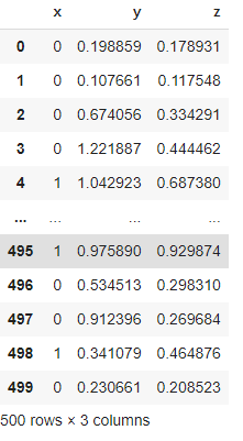
The above intuition says that if we have the information of potential outcomes we can easily estimate the ATE so in the next I am going to generate a data set where I have modelled the Y0 and Y1. and the success of modelling of counterfactual depends on the modelling of the Y0 and Y1. in this link you will get all the dataset generators which can be used for practising the causal inference. Considering the size of the article I am not posting the data generator codes here. By visualizing the data we can see the insights.

The above image is the representation of the data we have generated where y and z are our potential outcomes.

Let’s make a scatter plot to understand it more.

observed_data_1.plot.scatter(x="z", y="y", c="x", cmap="rainbow", colorbar=False);

Output:

Here we can see by this scatter plot that there is a very small difference between the groups and the distribution of Y.

sns.kdeplot(observed_data_1.loc[lambda df: df.x == 0].y)
sns.kdeplot(observed_data_1.loc[lambda df: df.x == 1].y)

Output:

By this density plot, we can say that there is a slight difference between the group lets check for the distribution of covariance Z for each group.

sns.kdeplot(observed_data_1.loc[lambda df: df.x == 0].z)
sns.kdeplot(observed_data_1.loc[lambda df: df.x == 1].z)

Output:

We can also confirm the difference by just looking at the difference in the mean of these groups.

print("Observed ATE: {estimated_effect:.3f} ({standard_error:.3f})".format(**estimate_uplift(observed_data_1)))

Output:

print("Real ATE:  {estimated_effect:.3f} ({standard_error:.3f})".format(**run_ab_test(generate_dataset_1)))

 Output:

Here, we have run an A/B test which we should not do because it is not feasible and impractical as we have discussed. To know the real ATE we can use any regression model. 

As we know the equation for a simple regression model is:

Y = α + βX

By just looking at the equation we can say it is a perfect fit for our model and using the linear regression we can estimate the ATE.

The package CausalInference gives the facility to perform this where we need only three values Y, D, and X.

from causalinference import CausalModel
cm = CausalModel(
    Y=observed_data_1.y.values, 
    D=observed_data_1.x.values, 
    X=observed_data_1.z.values)
cm.est_via_ols(adj=1)
print(cm.estimates)

 Output:

Here we can see that the model has given the estimation of the ATE and with this, we also have a confidence interval where the ATE is lying and according to that, we can say that we have got a correct ATE.

Note – we have modelled the data for good results. You may find some other results according to the complexity of the data.

Covariate Imbalance

Let’s think about a situation where we have data in which the covariance is in an imbalanced shape. We have data where we have only one type of sample in the data space at one time either treated or untreated. I have modelled the data for this again. There is the same link where readers can check it.

Let’s look at the scatter plot to understand the above-given high-dimensional situation.

observed_data_3.plot.scatter(x="z", y="y", c="x", cmap="rainbow", colorbar=False)

 Output:

print("Observed ATE: {estimated_effect:.3f} ({standard_error:.3f})".format(**estimate_uplift(observed_data_3)))

print("Real ATE:  {estimated_effect:.3f} ({standard_error:.3f})".format(**run_ab_test(generate_dataset_3)))

Output:

Let’s check the ATE estimation using OLS and Matching Estimator in the Causal Model.

# OLS estimator
cm = CausalModel(
    Y=observed_data_3.y.values, 
    D=observed_data_3.x.values, 
    X=observed_data_3.z.values)
cm.est_via_ols()
print(cm.estimates)

Output:

# Matching estimator
cm = CausalModel(
    Y=observed_data_3.y.values, 
    D=observed_data_3.x.values, 
    X=observed_data_3.z.values)
cm.est_via_matching()
print(cm.estimates)

Output:

Here we can see matching estimators are showing some improved results which means they are passed in capturing the true effect of covariant but the OLS estimators are not giving that much proper results. We can see this issue regularly if we start looking for covariance in the high dimensional data. Also, we have an option in the Causalnference package to check for the summary.

print(cm.summary_stats)

Output:

Here in the summary, the normalized difference represents the overlapping between the covariate and if the value of it is greater than one which means there is not so much overlapping also we have seen this in the scatter plot.

Propensity Score

When the covariates are given the propensity is an estimation of the likelihood for a subject that has ended up with the treatment.

p^(Z)=P(X|Z)

Estimating propensity score can help measure many things in causal inference one of them is the inverse propensity score weight estimator.

We can estimate the propensity using the causalinference package. Let’s do this on the observed_data_1. Which we have used before in the examples.

cm = CausalModel(
    Y=observed_data_1.y.values, 
    D=observed_data_1.x.values, 
    X=observed_data_1.z.values)
cm.est_propensity_s()
propensity = cm.propensity["fitted"]
propensity 

Output:

Measuring the causal inference was about Know the value of E[Yi], which can be estimated by

E[Yi]=E[(Yi / P(X=i|Z)) P(X=i|Z)] 

Here we have an inverse propensity in the formula so the propensity we measured if we inverse it and weight each point the result will be called the inverse propensity score weight estimator.

Inverse propensity score weight estimator:

df = observed_data_1
df["ips"] = np.where(
    df.x == 1, 
    1 / propensity,
    1 / (1 - propensity))
df["ipsw"] = df.y * df.ips
ipse = (
      df[df.x == 1]["ipsw"].sum()
    - df[df.x == 0]["ipsw"].sum()
) / df.shape[0]
ipse

Output:

We have got a good result for our dataset. The inverse propensity score weight estimator depends on the goodness of the estimation of the propensity score.

Unconfoundedness and the Propensity Score

In the last sections of the article, we have assumed that the potential outcomes Y0 and Y1 are independent of the X and Z. here in this section we are making one more assumption about the potential outcomes that they are also independent of the propensity score.

The assumption we have made here will help us in the reduction of the confounding variable’s dimensionality. Using this reduction we can perform several techniques. Like trimming and stratification.

Trimming

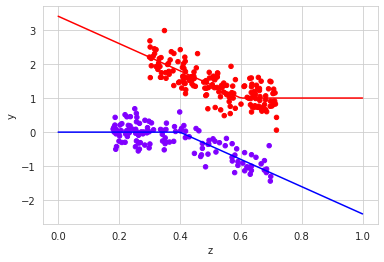
In the observed_data_3 we have seen that we had a problem of imbalance covariants which can be solved by a good overlap or trim and the data we have used having almost zero overlap lets see how we can solve this issue by trimming

Older structure of the dataset:

observed_data_3 = generate_dataset_3()
observed_data_3.plot.scatter(x="z", y="y", c="x", cmap="rainbow", colorbar=False)
# actual response curves
z = np.linspace(0,1,100)
y0 =  np.where(z >= 0.4, -4*(z - 0.4), 0)
y1 =  np.where(z < 0.6,  -4*(z - 0.6), 0) + 1
plt.plot(z,y0, "b")
plt.plot(z,y1, "r")

Output:

Trimming the data based on the propensity score:

Data structure after trimming:

# mask out data ignored by them
propensity = cm.propensity["fitted"]
cutoff = cm.cutoff
mask = (propensity > cutoff) &  (propensity < 1 - cutoff)
# plot the data
observed_data_3[mask].plot.scatter(x="z", y="y", c="x", cmap="rainbow", colorbar=False)
# actual response curves
z = np.linspace(0,1,100)
y0 =  np.where(z >= 0.4, -4*(z - 0.4), 0)
y1 =  np.where(z < 0.6,  -4*(z - 0.6), 0) + 1
plt.plot(z,y0, "b")
plt.plot(z,y1, "r")

Output:

Checking for the observed and real ATE

filter_ = lambda df: (df.z > 0.2) & (df.z < 0.7)
print("Observed ATE: {estimated_effect:.3f} ({standard_error:.3f})".format(**estimate_uplift(observed_data_3[mask])))
print("Real ATE:  {estimated_effect:.3f} ({standard_error:.3f})".format(
    **run_ab_test(dg.generate_dataset_3, filter_= filter_)))

Output:

Here we can see that we have got a good result. Basically, by trimming we can measure the causal inference for some part of the covariate space.

Stratification

We have seen there are various propensity scores when we generate the propensity but we can divide them into groups based on the similarity and stratification or blocking allow us to put the data points into the groups of propensity scores.

We can stratify the data points using the package causalInference.

These groups can be used for measuring the overall ATE. 

cm.est_via_blocking()
print(cm.estimates)

 Output:

We can see that we have got a good result again.

Final Words

Here in the article, we have revolved around the estimation of ATE and we have found that various techniques of estimating have their inference and place where we can apply them. The data we have used in the analysis is observational data. Ultimately we can say that if we have good covariate space the matching technique is better because only in ideal data we do have no opposite treatment point in the focus space of data. When such conditions are not there we can use any of the methods or iterate all of them for good results.

• Causal Inference package in Python
• Google Colab notebook for codes
• Google Colab notebook for data generators
• Causal inference
• Causal Inference Notes