A Guide to VARMA with Auto ARIMA in Time Series Modelling

Share

Published on September 28, 2021

by Yugesh Verma

Listen to this story

Time series modelling needs a series of steps to be performed such as processing the time series data, analyzing the data before modelling with different types of tests and then finally modelling with the data. There are different types of tests and modeling techniques used based on the types of requirements. There are different modelling techniques based on the Moving Average (MA) of the time series, each of them has its own advantages. Here in this article, we are going to discuss such a model named VARMA (Vector Auto Regressive Moving Average) and we will see how it can be implemented with the Auto-ARIMA model to achieve some specific types of results. The major points to be covered in this article are listed below.

What is ARIMA?
Why Do We Need Auto-ARIMA?
What Is VARMA(Vector Auto Regressive Moving Average)?
What is VARMA With Auto ARIMA?
Implementing VARMA With Auto ARIMA

Let us begin with understanding the ARIMA model.

What is ARIMA?

Before going for the Auto-ARIMA we need to understand what the ARIMA model is? In time series analysis, the ARIMA model is a model made up of three components: Auto-Regressive(AR), Integrated(I), and Moving Averages(MA).

p: Stands for the number of lag observations included in the model, also known as the lag order.
d: The number of times the raw observations are differentiated, also called the degree of difference.
q: Is the size of the moving average window and also called the order of moving average.

Before implementing the ARIMA model it is assumed that the time series we are using is a stationary time series and a univariate time series. To work with the ARIMA model we need to follow the below steps:

Load the data and preprocess the data.
Check the stationarity of the data.- if stationary then proceed for the further steps and if not then make it stationary.
determine the degree of differencing(d).
Determine the order of lag(p) and moving average(q), which can be done by making a PACF(partial autocorrelation function) and ACF(autocorrelation function) plot.
Fitting the model and making the prediction.
Check the performance of the model by calculating RMSE(root mean square error) between the actual and predicted values.

So hereby the full procedure we can understand that following all the steps can become time-consuming. You can check the full implementation of an ARIMA model in this article. To save us from this situation auto-ARIMA comes into the picture.

Why do we need Auto-ARIMA?

As we know, ARIMA models are a very powerful tool for us in time series analysis but on the other hand, we are required to analyze model prediction on the basis of p, q, and d values here Auto-ARIMAis a model using which we can save our time in iterating between the p,q and d values. It helps in finding the best combination of these values and fitting them into the ARIMA model. A combination of these values can be estimated by estimating the AIC (Akaike information criterion) and BIC(Bayesian Information Criterion). Lower AIC and BIC values give the best combination of p, q, and d. Here, by providing the best combination, the Auto-Arima model saves us from performing some of the steps in the ARIMA modelling procedure.

In the above, we learned that an ARIMA or Auto-ARIMA model is a powerful tool when working with the univariate time series. So when we talk about a multivariate time series VARIMAX models come into the picture.

What is VARMA (Vector Auto Regressive Moving Average)?

When the scenario comes on the modelling for a multivariate time series we can use different models like VAR and VMA and VARMA. The Vector Auto-Regressive(VAR) model is a generalization of the auto-regressive model for multivariate time series where the time series is stationary and we consider only the lag order ‘p’ in the modelling. The Vector Moving Average(VMA) model is a generalization of the Moving Average Model for multivariate time series where the time series is stationary and we consider only the order of moving average ‘q’ in the model.

The Vector Autoregressive Moving Average(VARMA) model is a combination of VAR and VMA models that helps in multivariate time series modelling by considering both lag order and order of moving average (p and q)in the model. We can make a VARMA model act like a VAR model by just setting the q parameter as 0 and it also can act like a VMA model by just setting the p parameter as 0.

What is VARMA With Auto ARIMA?

From the above-given information, we can understand what is going to happen next in the article. As we have discussed, ARIMA is time-consuming because of the procedure for finding the best combination of parameters p,q, and d and which makes us introduce the auto-ARIMA model which helps in finding the best-fit combination of parameters for better performance of the model.

Here we have the VARMA model where we have two parameters p and q, again if we go with the simple model obviously we will find it problematic in case of finding the best combination of parameters for better performance of the model. In these situations, we can try a model from which we can get the combination of p and q parameters easily and without wasting time in iteration with random parameters we can fit them in the VARMA model and increase the performance of the model in less time. So here we try to find the best-fit combination of the parameters by Auto-ARIMA and we use those parameters in the VARMA model for predicting the forecast values.

Let’s see how we can implement this. To reduce the size of the article, many of the coding parts are presented in brief. For complete codes of VARMA with Auto ARIMA, you can check out this link to find the Colab notebook.

Implementing VARMA With Auto ARIMA

First of all, we are importing some of the basic libraries which we will require in the procedure. So that we can know these packages are installed in our system.

import pandas as pd
import matplotlib.pyplot as plt
from statsmodels.tsa.statespace.varmax import VARMAX
import numpy as np
from statsmodels.tsa.stattools import adfuller
from sklearn import metrics
from timeit import default_timer as timer
import warnings
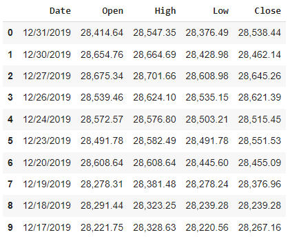
warnings.filterwarnings("ignore")

I am using the Dow_jones_Industrial_average data where we have an opening, closing, and high and low information of the shares of the Dow Jones industries. The reader can get this data from this link.

10 head values of the data are as follows:

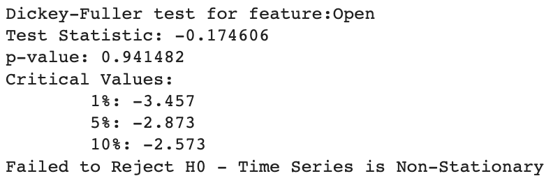
As we have discussed, to perform ARIMA modelling first we need to check whether the time series is stationary or not. I will perform a dickey-fuller test to check the stationarity of the four series. To know more about the test, you can go to this link.

So the results of the test are as follows:

Dickey-Fuller Test for Open

Dickey-Fuller Test for High

Dickey-Fuller Test for Low

Dickey-Fuller Test for Close

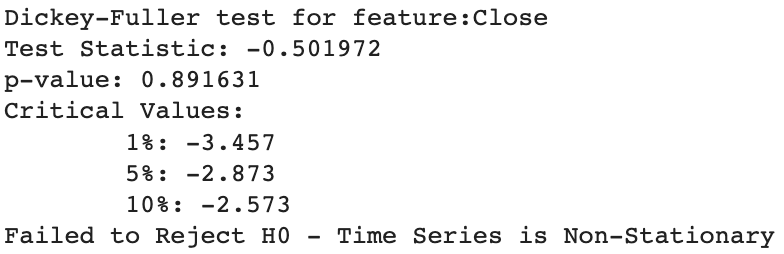
Here we can see that the series of data is not stationary in the Dickey-Fuller test we measure the p-value for the series in the value is lower than 0.02 then we can say the time series is stationary and if the p-value is greater than 0.02 which states that time series is not stationary.

So here we need to make the time series stationary. There can be many methods to make the data stationary some of them are

Detrending
Seasonal adjustment
Transformation

To make it stationary I am using a differencing method which comes under the transformation methods. Where we just subtract a time series value from its only one lagged value. After differencing the dickey fuller test results are as follows:

Dickey-Fuller Test for Open after Differencing

Dickey-Fuller Test for High after Differencing

Dickey-Fuller Test for Low after Differencing

Dickey-Fuller Test for Close after Differencing

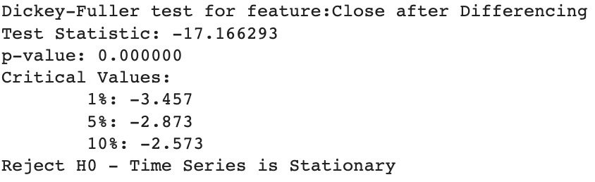
Here we can see all the series in the data set are now stationary. After this, we can perform the Johansen cointegration test in multivariate time series to see if the series is correlated to each other or not.

The Johansen cointegration test results are as follows:

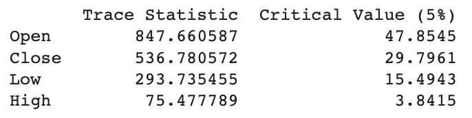
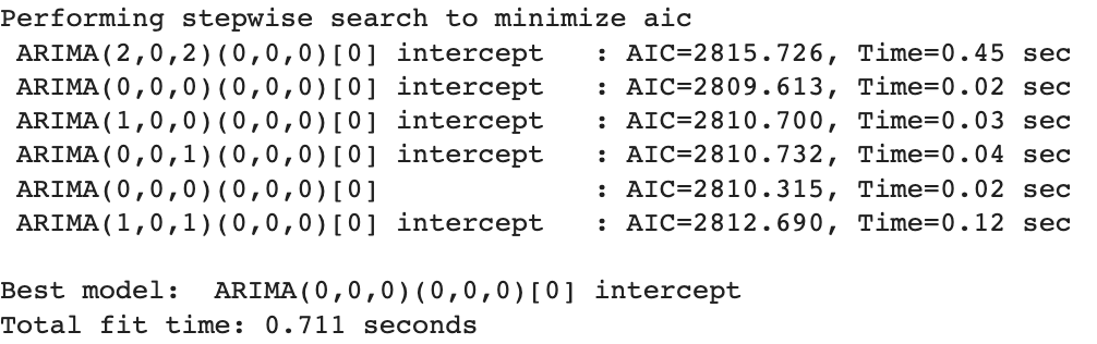
Here we can see that the multivariate time series we are using are correlated. Now we can apply the Auto ARIMA model. Which will tell us the order of p and q for our VARMA model. To apply the Auto-ARIMA model on time series data using the prima library. We can import the model for Auto-ARIMA like this

from pmdarima import auto_arima

The results for p and q are as follows:

Order of p and q for Open

Order of p and q for High

Order of p and q for Low

Order of p and q for Close

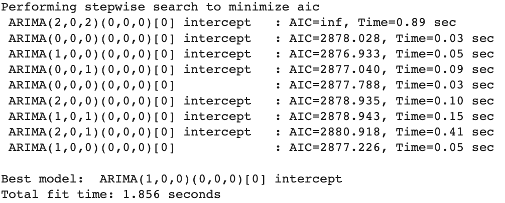
Here these four optimal orders can be divided into two parts because we can not give the order of q as 0 and we can see that we have order values for high and low values of the stock. So here we should iterate the VARMA model between (1,0,1) and (1,0,0).

As we have talked about, our major concern for this modelling is to save our time from iterating the model with different p and q values. We can see in the above outputs that we have various values for p and q order. Finding them all from PACF and ACF plots could consume so much time. Now we have only two combinations and iterating the model for these two combinations took the following effort

So the picture is clearer now by analyzing the RMSE score we can say that orders of p = 0 and q = 1 will give the best score and forecasting values for this multivariate time series.

We can fit the model on a time series with p=0 and q=1 combinations. The forecasting results are as follows.

Forecasting Results for High

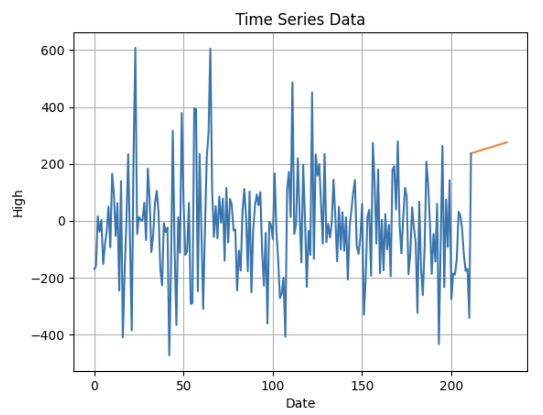
Here we can see our results which are very satisfactory. The codes for all this implementation are given in this link.

Final Words

In this article, we have seen what ARIMA is, why we use Auto ARIMA and how we can use the Auto ARIMA model with the VARMA model. The major points that we focused on in the article are the p, q, and d values. With them, we are required to learn how we can make the best combination of these values. Since Auto ARIMA makes this procedure of finding combinations easy for us, I suggest you find the combinations by analyzing the PACF and ACF plots also. These are very basic things which we should know about before going to understand the advanced techniques. There are various things and techniques that I used in the article that are not deeply explained. Below are the links to a few articles that will give you a deep understanding of those things.

References

Access all our open Survey & Awards Nomination forms in one place