


There are many different complex and simple algorithms available to Data Scientists, in classification, a particularly simple algorithm managed to do wonders in ML applications. The Naive Bayes classification algorithm has been in use for a very long time, particularly in applications that require classification of texts. It is a probabilistic algorithm based on the popular Conditional Probability and Bayes Theorem.
The Bayes Theorem
The Bayes theorem has various applications in Machine Learning, categorizing a mail as spam or important is one simple and very popular application of the Bayes classification.
One of the simplest definitions of the Bayes Theorem is that it describes the probability of an event, based on prior knowledge of conditions that might be related to the event.
The theorem is mathematically expressed as :

Where A and B are events and P(B) is never zero :
P(A|B) is the likelihood of event A occurring given that B is true.
P(B|A) is the likelihood of event B occurring given that A is true.
P(A) and P(B) are the probabilities of observing A and B independently of each other.
Click here for more explanation and examples.
Lets Code!
Getting the dataset
In the following code section, we will use a classification dataset from Machinehack’s Predict The Data Scientists Salary In India Hackathon.
To get the dataset, head to Machinehack, Sign up, start the hackathon and download the dataset from the hackathons attachment page.
Having trouble finding the data set? Click here to go through the tutorial to help yourself.
For simplicity, we will only be using a smaller subset of the dataset provided by Machinehack.
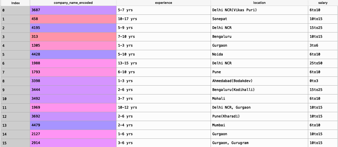
Shown below is the data we will deal with in the proceeding code:
Python Code For Naive Bayes Classification
Importing the Dataset
import pandas as pd

data = pd.read_csv("Final_Train_Dataset.csv")

data = data[['company_name_encoded','experience', 'location', 'salary']]
The above code block will give a new data set as shown in the image above.
Exploring The Dataset
print("#"30)

print("\nFeatures/Columns : \n", data.columns)

print("#"30)

print("\n\nNumber of Features/Columns : ", len(data.columns))

print("#"30)

print("\nNumber of Rows : ",len(data))

print("#"30)

print("\n\nData Types :\n", data.dtypes)

print("#"30)

print("\nContains NaN/Empty cells : ", data.isnull().values.any())

print("#"30)

print("\nTotal empty cells by column :\n", data.isnull().sum(), "\n\n")

print("#"30)

print("\n\nNumber of Unique Locations : ", len(data['location'].unique()))

print("#"30)

print("\n\nNumber of Unique Salaries : ", len(data['salary'].unique()))

print("#"30)

print("\n\nUnique Salaries:\n", data['salary'].unique())

print("#"30)
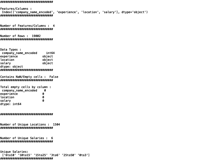
The above code block is to help us understand the kind of data we are dealing with such as the number of records or samples, number of features, presence of missing values, unique classes etc
Output :
Cleaning The Data
Now let us clean up the data.
We can see that the experiences are given in strings, so lets convert them to integers in a logical way by splitting it in to minimum experience (minimum_exp) and maxim experience (maximum_exp).Also we will label encode the categorical features location and salary. We will then delete the original experience column, attach the new ones.
#Cleaning the experience

exp = list(data.experience)

min_ex = []

max_ex = []
for i in range(len(exp)):

exp[i] = exp[i].replace("yrs","").strip()

min_ex.append(int(exp[i].split("-")[0].strip()))

max_ex.append(int(exp[i].split("-")[1].strip()))
#Label encoding location and salary

from sklearn.preprocessing import LabelEncoder

le = LabelEncoder()data['location'] = le.fit_transform(data['location'])

data['salary'] = le.fit_transform(data['salary'])
#Attaching the new experiences to the original dataset

data["minimum_exp"] = min_ex

data["maximum_exp"] = max_ex
#Deleting the original experience column and reordering
data.drop(['experience'], inplace = True, axis = 1)
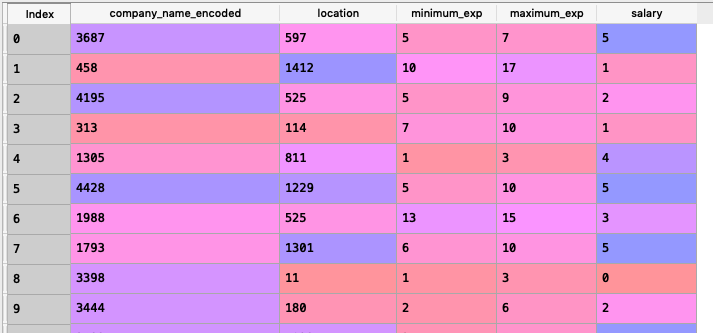
data = data[['company_name_encoded', 'location','minimum_exp', 'maximum_exp', 'salary']]
After executing all the above code blocks our new dataset will look like this:
Feature Scaling
We will now scale all the numerical features in the dataset except the target variable which is salary(category).
from sklearn.preprocessing import StandardScaler

sc = StandardScaler()

data[['company_name_encoded', 'location', 'minimum_exp', 'maximum_exp']] = sc.fit_transform(data[['company_name_encoded', 'location', 'minimum_exp', 'maximum_exp']])
After scaling the dataset will look like what is shown below :

Creating training and validation sets
#Splitting the dataset into  training and validation sets

from sklearn.model_selection import train_test_split

training_set, validation_set = train_test_split(data, test_size = 0.2, random_state = 21)

#classifying the predictors and target variables as X and Y

X_train = training_set.iloc[:,0:-1].values

Y_train = training_set.iloc[:,-1].values

X_val = validation_set.iloc[:,0:-1].values

y_val = validation_set.iloc[:,-1].values
The above code block will generate predictors and targets which we can fit our model to train and validate.
Measuring the Accuracy
We will use confusion matrix to determine the correct number of predictions. The accuracy is measured as the total number of correct predictions divided by the total number of predictions. We will define a function to calculate and return the accuracy.
def accuracy(confusion_matrix):

diagonal_sum = confusion_matrix.trace()

sum_of_all_elements = confusion_matrix.sum()

return diagonal_sum / sum_of_all_elements
Initialising the Naive Bayes Classifier
We now have all the data ready to be fitted to the Bayesian classifier. In the below code block we will initialize the Naive Bayes Classifier and fit the training data to it.
#Importing the library

from sklearn.naive_bayes import GaussianNB

#Initializing the classifier

classifier = GaussianNB()

#Fitting the training data

classifier.fit(X_train, Y_train)
Predicting for the validation set
The below code will store the predictions returned by the predict method into y_pred
y_pred = classifier.predict(X_val)
Generating the confusion matrix and printing the accuracy
The below-given code block will generate a confusion matrix from the predictions and the actual values of the validation set for salary.
#Generating the confusion Matrix

from sklearn.metrics import confusion_matrix
cm = confusion_matrix(y_val, y_pred)
print("__ACCURACY = ", accuracy(cm))
Output :
__ACCURACY = 0.48351276881154321
The Naive Bayesian classifier when fitted with the given data gave an accuracy of 48%.