

Survival analysis is a part of statistics where the expected duration of time for the occurrence of any event is analyzed. It is used for various purposes such as duration analysis in economics, event history analysis in sociology, etc. This analysis is done for answering the questions like what portion of the population will survive in a certain time, the portion which is surviving at what rate they will fail or die, what causes of death can be taken into account, etc. This analysis helps in studying the reliability of any system which is going to close or destroy one day. In this article, we will discuss the survival analysis in detail along with its concepts including proportional hazards models and time-varying effects. We will also perform a survival analysis on the real-life data in Python. The major points to be covered in this article are listed below.
Table of Contents
- Introduction to the Data
- What is Survival Analysis?
- Bayesian Proportional Hazards Models
- Time-Varying Effects
Introduction to the Data
Our analysis is survival analysis where we will take a look at how the expected duration of time is distributed until one event occurs. That can be used in many fields like economics, biology, social science etc. in this article we will try to fit and analyze the Bayesian survival model in Python using the package PyMC3 and mastectomy dataset provided in the link. Some of the values from the data set are shown below for understanding.

Each observation represents a woman patient diagnosed with breast cancer who had gone through a mastectomy. Time represents the time duration in months of post-surgery and the event is an indication of a woman’s situation whether she is alive or died during the observation period. The column metastasized represents whether cancer had metastasized or not
Next in the article, we will analyze the relationship between survival time and mastectomy.
What is Survival Analysis?
We can consider survival analysis as a branch of statistics if we are interested in analyzing the occurrence of any event in the expected duration of time. Let’s talk about our used example where We are interested in analyzing the time taken by women for death while they are dealing with breast cancer and have gone through the mastectomy.
Some of the common functions used in survival analysis are:
Survival function: it is a function used to give the probability of any object in which we are interested to know if it will survive beyond any specified time or not. In our case the objects are women. Mathematically it can be given by

Where S(t) is a survival function in which T is a continuous random variable and the time for an interesting event. The F(t) is a cumulative distribution function on the interval[0,∞).
We can also write the survival function in terms of the hazard rate. The hazard rateλ(t) is the major of the instantaneous probability of occurrence of an event at time t, given that it has not yet occurred.
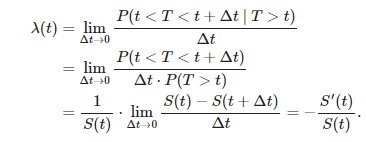
Above given hazard rate can help in calculating the survival function:
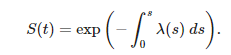
Where,
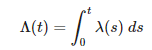
is a cumulative hazard function
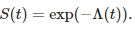
So consecutively we can say and formulate the survival function as:
One more important point to notice in the survival analysis is censoring. In our example there are two types of women. one type is those who are observed as dead where the event has the value 1 and the second type are those who are observed as not dead yet and the event has the value 0. Since we do not have every sample in the data as died, in the data there are some samples that represent observations in which women are thankfully alive in these data samples which are alive at a point in time can be considered as censored and those who are not alive represent the uncensored data.
Let’s take a look at the mean of the event column of the data which is obtained as:
Hereby we can say that 40% of the data is censored. Let’s make a visualization so that things will be more clear.
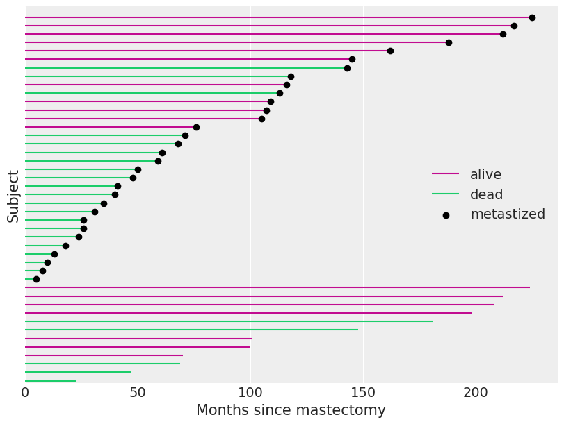
Here we have all the details of our observation which are dead or alive and have gone through the mastectomy observation or not. By this visualization, we can say that if the observation where the value of the event column is zero or the woman is alive the time given in the data is not the survival time and in conclusion, we can say that the true survival time of the subject exceeds the time in the data.
Bayesian Proportional Hazards Models
Generally, two Bayesian estimators are used in survival analysis:
- Kaplan-Meier estimator for the survival function
- the Nelson-Aalen estimator for cumulative hazard function.
Since our requirement is to understand the impact of metastasized on survival time, a risk regression model (Cox’s proportional hazards model) can be used in the process.. In the model, with the covariates x and regression coefficients βt, hazard rate can be written as:
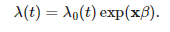
Here λ0(t) is the baseline hazard, which is independent of the covariates. In our example, we can assume the metastasized values as the covariate for the hazard rate.
Here to make Bayesian inference with this model, we must specify priors on regression coefficients β and baseline hazard rate λ0(t). Here we are specifying a normal prior as β∼N(μβ,σβ2), where μβ∼N(0,10^2) and σβ∼U(0,10). And specifying a semi-parameter prior to baseline hazard.
Specified prior to baseline hazard will be required to make partition of time range into different intervals. If 0≤s1<s2<⋯<sN. Are the partitions, the baseline hazard will be λ0(t)=λj where sj≤t<sj+1. With λ0(t) constrained to have this form, all we need to do is choose priors for the N−1 values λj. We use independent vague priors λj∼Gamma(10−2,10−2).
Here in our example, we will make each such partition where the interval of time is three months long. Let’s take a look at the below graph
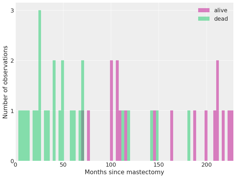
It is a representation of the count of dead and alive people on the partitioned time intervals. Now after specifying the priors on the hazard and regression coefficients we can fit the models. Here one thing is noticeable that the hazard model is closely related to the Poisson model where the likelihood function makes the difference between them in the Poisson model. It depends on the data, not on the regression coefficient and baseline hazard.
Before fitting the model we are required to specify one more thing on the subjects if they died in the jth interval (as 1) otherwise no one died in the interval (as 0) so that we can know the risk factor on the jth interval of dying people.
We can formulate the risk incurred of the ith subject at jth time interval as
λi,j = λjexp(xiβ)
The below image gives the representation of the model fitting on the data.
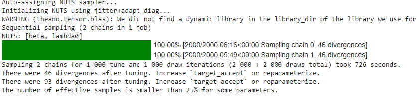
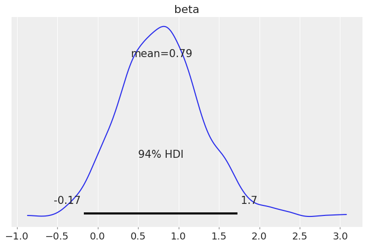
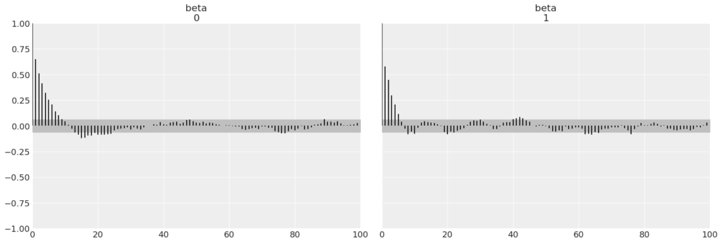
We see in the image the hazard rate for women who are metastasized is about one and approx a half times the rate of those whose cancer has not metastasized. Below the graphs are posterior distribution and the autocorrelation graphs of the regression coefficients of the model.
Now we can examine the effects on the survival function and the cumulative hazard by the metastasized
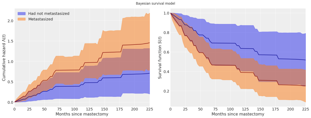
In the above image, we can see that the initial points of the cumulative hazard for metastasized women are increasing more than the baseline hazard but after some time cumulative hazard and baseline hazard are behaving parallel to each other.
Time-Varying Effects
In the above model, we have seen that cumulative hazard is varying over time because of metastasization or we can say that after the metastasized there is an increase in the hazard rate which is immediately after the mastectomy and the risk is decreasing after the metastasized. We can use this inference in the model. This is just because we have seen that the regression coefficient is varying over time.
In the time-varying coefficient model, if sj≤t<sj+1 we let λ(t)=λjexp(xβj). The sequence of regression coefficients β1,β2,…,βN−1 form a normal random walk with β1∼N(0,1)
, βj | βj−1∼N(βj−1,1)
.
Let’s see on the below graph
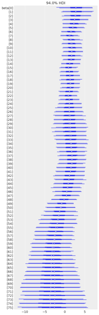
From the plot we can say that initially βj>0, indicates an elevated hazard rate due to metastasized, but that this risk declines as a βj<0 eventually.
Let’s have a look at the below graph:
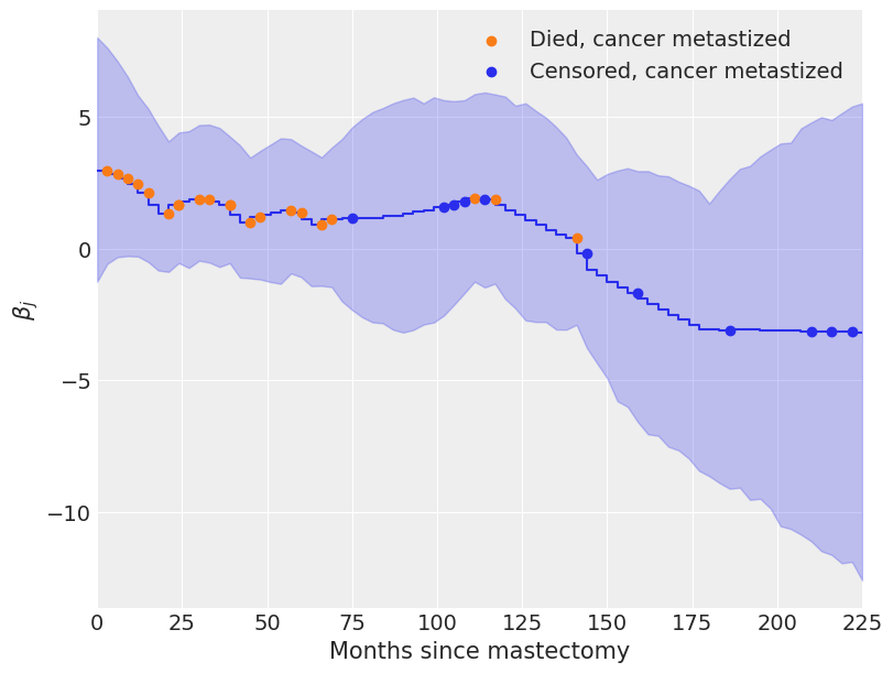
Here we can see that the value of the regressive coefficient is decreasing after the 100th month which means only three of the women have died after the mastectomy of their cancer; the risk of being dead is reduced.
Let’s make a visualization for cumulative hazard and survival functions for this model where the time-varying effect is included with the comparison of the old model where the regression coefficient was stable.
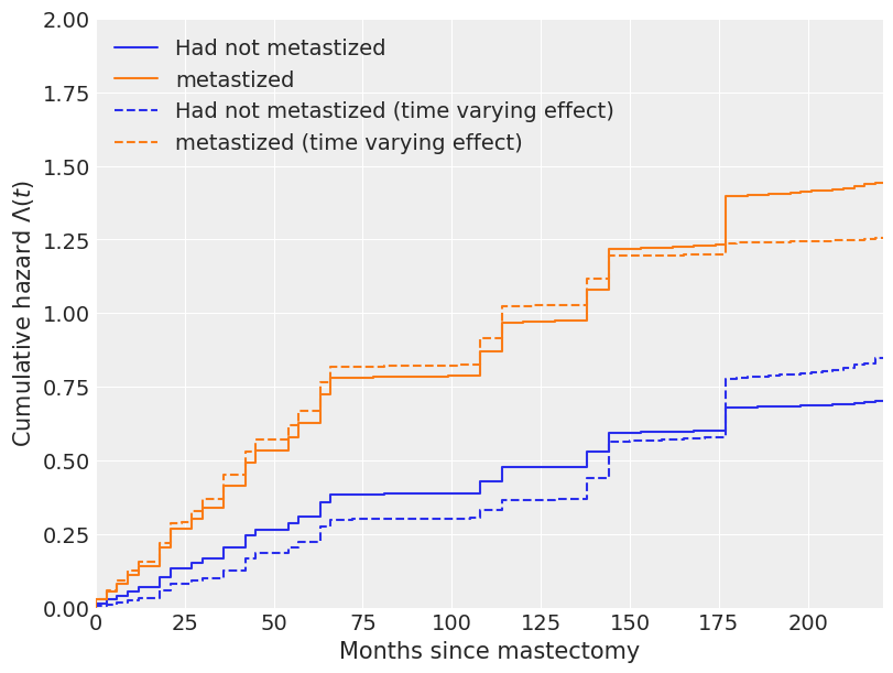
Here we can see we’ve got some changes in the plots after considering the time-varying effect now we have more space for our prior than before. Which is quite good. We require that space in our model for better and accurate analysis.
The below plot is a representation of the cumulative hazard and survival function of the model where we included the time-varying effects.

Here we can see that we have stretched the space more than the survival analysis.
Final Words
Here we have completed our analysis in which we have seen that when we were doing the survival analysis we have also considered the hazard rate as our major concern in analysis. Here we have considered a stable regression inference and when we have chosen the regression coefficients as the subject of time we have got some more space to perform the analysis in the data.
References: