

In the era of data science and machine learning, various machine learning concepts are used to make things easier and profitable. When it comes to marketing strategies it becomes very important to learn the behaviour of different customers regarding different products and services. It can be any kind of product or service the provider needs to satisfy the customers to make more and more profits. Machine learning algorithms are now capable of making inferences about consumer behaviour. Using these inferences a provider can indirectly influence any customer to buy more than he wants.
Arranging items in a supermarket to recommend related products on E-Commerce platforms can affect the profit level for providers and satisfaction level for consumers. This arrangement can be done mathematically or using some algorithms. In this article we are going to discuss the two most basic algorithms of market basket analysis, one is Apriori and the other one is FP-Growth. The major points to be discussed in this article are listed below.
Table of content
- Association Rule Learning
- Frequent Itemset Mining(FIM)
- Apriori
- FP-Growth
- Comparing Apriori and FP-Growth
Let us understand these concepts in detail.
Association Rule Learning
In machine learning, association rule learning is a method of finding interesting relationships between the variables in a large dataset. This concept is mainly used by supermarkets and multipurpose e-commerce websites. Where it is used for defining the patterns of selling different products. More formally we can say it is useful to extract strong riles from a large database using any measure of interestingness.
In supermarkets, association rules are used for discovering the regularities between the products where the transaction of the products are on a large scale. For example, the rule {comb, hair oil}→{mirror} represents that if a customer is buying comb and hair oil together then there are higher chances that he will buy the mirror also. Such rules can play a major role in marketing strategies.
Let’s go through an example wherein in a small database we have 5 transactions and 5 products like the following.
| transaction | product1 | product2 | product3 | product4 | product5 |
| 1 | 1 | 1 | 0 | 0 | 0 |
| 2 | 0 | 0 | 1 | 0 | 0 |
| 3 | 0 | 0 | 0 | 1 | 1 |
| 4 | 1 | 1 | 1 | 0 | 0 |
| 5 | 0 | 1 | 0 | 0 | 0 |
Here in the database, we can see that we have different transaction id for every transaction and 1 represents the inclusion of the product in the transaction, and 0 represents that in the transaction the product is not included. Now in transaction 4, we can see that it includes product 1, product 2, and product 3. By analyzing this we can decide a rule {product 2, product 3} →{product 1}, where it will indicate to us that customers who are buying product 2 and product 3 together are likely to buy product 1 also.
To extract a set of rules from the database we have various measures of significance and interest. Some of the best-known measures are minimum thresholds on support and confidence.
Support
Support is a measure that indicates the frequent appearance of a variable set or itemset in a database. Let X be the itemset and T a set of transactions in then the support of X with respect to T can be measured as

Basically, the above measure tells the proportion of T transactions in the database which contains the item set X. From above the given table support for itemset {product 1, product 2} will be ⅖ or 0.4. Because the itemset has appeared only in 2 transactions and the total count of transactions is 5.
Confidence
Confidence is a measure that indicates how often a rule appears to be true. Let A rule X ⇒ Y with respect to a set of transaction T, is the proportion of the transaction that contains X and Y at the same transaction, where X and Y are itemsets. In terms of support, the confidence of a rule can be defined as
conf(X⇒Y) = supp(X U Y)/supp(X).
For example, in the given table confidence of rule {product 2, product 3} ⇒ {product 1} is 0.2/0.2 = 1.0 in this database. This means 100% of the time the customer buys product 2 and product 3 together, product 1 bought as well.
So here we have seen the two most known measures of interestingness. Instead of these terms, we have some more measures like lift conviction, all confidence, collective strength, and leverage which have their meaning and importance. This article is basically dependent on having an overview of the techniques of frequent itemset mining. Which we will discuss in our next part.
Frequent Itemset Mining(FIM)
Frequent Itemset Mining is a method that comes under the market basket analysis. Above in the article, we have an overview of the association rules which tells us how rules are important for market basket analysis in accordance with the interestingness. Now in this part, we will see an introduction to Frequent Itemset mining which aims at finding the regularities in the transactions performed by the consumers. In terms of the supermarket, we can say regularities in the shopping behaviour of customers.
Basically, frequent itemset mining is a procedure that helps in finding the sets of products that are frequently bought together. Found frequent itemsets can be applied on the procedure of recommendation system, fraud detection or using them we can improve the arrangement of the products in the shelves.
The algorithms for Frequent Itemset Mining can be classified roughly into three categories.
- Join-Based algorithm
- Tree-Based algorithms
- Pattern Growth algorithms
Where the join based algorithms expand the items list into a larger itemset to a minimum threshold support value which defines by the user, the tree-based algorithm uses a lexicographic tree that allows mining of itemsets in a variety of ways like depth-first order and the pattern growth algorithms make itemsets depends on the currently identified frequent patterns and expand them.
Now we can classify and find frequent itemset using the following algorithms:

Next in the article will have an overview of a classical Apriori Algorithm and FP Growth Algorithm.
Apriori
The apriori algorithm was proposed by Agrawal and Srikant in 1994. It is designed to work on the database which consists of transaction details. This algorithm finds ( n + 1) itemsets from n items by using an iterative level-wise search technique. For example, let’s take a look at the table of transaction details of the 5 items.
| Transaction ID | List of items |
| T100 | I1, I2, I5 |
| T200 | I2, I4 |
| T300 | I2, I3 |
| T400 | I1, I2, I4 |
| T500 | I1, I3 |
| T600 | I2, I3 |
| T700 | I1, I3 |
| T800 | I1, I2, I3, I5 |
| T900 | I1, I2, I3 |
In the process of Frequent Itemset Mining, the Apriori algorithm first considers every single item as an itemset and counts the support from their frequency in the database, and then captures those who have support equal to or more than the minimum support threshold. In this process extraction of each frequent itemset requires the scanning of the entire database by the algorithm until no more itemsets are left with more than the minimum threshold support.

In the above image, we can see that the minimum support threshold is 2 so in the very first step items with support 2 are considered for the further steps of the algorithms. And in the further steps also it is sending the item sets having minimum support count 2, for further processing.
Let’s see how we can implement this algorithm using python. For implementation, I am making a dataset of 11 products and using the mlxtend library for making a Frequent dataset using the apriori algorithm.
dataset = [['product7', 'product9', 'product8', 'product6', 'product4', 'product11'],
           ['product3', 'product9', 'product8', 'product6', 'product4', 'product11'],
           ['product7', 'product1', 'product6', 'product4'],
           ['product7', 'product10', 'product2', 'product6', 'product11'],
           ['product2', 'product9', 'product9', 'product6', 'product5', 'product4']]
Importing the libraries.
import pandas as pdfrom mlxtend.preprocessing import TransactionEncoder
Making the right format of the dataset for using the apriori algorithm.
con = TransactionEncoder()
con_arr = con.fit(dataset).transform(dataset)
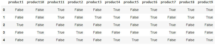
df = pd.DataFrame(con_arr, columns = con.columns_)
dfOutput:
Next, I will be making itemsets with at least 60% support.
from mlxtend.frequent_patterns import apriori
apriori(df, min_support=0.6, use_colnames=True)
Output:

Here we can see the itemsets with minimum support of 60% with the column indices which can be used for some downstream operations such as making marketing strategies like giving some offers in buying combinations of products.
Now let’s have a look at FP Growth Algorithm.
Frequent Pattern Growth Algorithm
As we have seen in the Apriori algorithm that it was generating the candidates for making the item sets. Here in the FP-Growth algorithm, the algorithm represents the data in a tree structure. It is a lexicographic tree structure that we call the FP-tree. Which is responsible for maintaining the association information between the frequent items.
After making the FP-Tree, it is segregated into the set of conditional FP-Trees for every frequent item. A set of conditional FP-Trees further can be mined and measured separately. For example, the database is similar to the dataset we used in the apriori algorithm. For that, the table of every conditional FP-Tree will look like the following.
| item | Conditional pattern base | Conditional FP-Tree | Frequent pattern generated |
| I5 | {{I2, I1: 1}, {I2, I1, I3: 1}} | {I2: 2, I1: 2} | {I2, I5: 2}, {I1, I5: 2}, {I2, I1, I5: 2} |
| I4 | {{I2, I1: 1}, {I2: 1}} | {I2: 2} | {I2, I4: 2} |
| I3 | {{I2, I1: 2}, {I2: 2}, {I1: 2}} | {I2: 4, I1: 2}, {I1: 2} | {I2, I3: 4}, {I1, I3: 4}, {I2, I1, I3: 2} |
| I1 | {{I2: 4}} | {I2: 4} | {I2, I1: 4} |
Based on the above table, the image below represents the frequent items as following:

Here we can see that the support for I2 is seven. Where it came with I1 4 times with I3, 2 times, and with I4 it came one time. Where in apriori algorithm was scanning tables, again and again, to generate the frequent set, here a one time scan is sufficient for generating the itemsets.
The conditional FP-Tree for I3 will look like the following image.

Let’s see how we can implement it using python. As we did above, again we will use the mlxtend library for the implementation of FP_growth. I am using similar data to perform this.
from mlxtend.frequent_patterns import fpgrowth
frequent_itemsets = fpgrowth(df, min_support=0.6, use_colnames=True)
frequent_itemsets
Output:

Here we can see in comparison of apriori where the frequent itemset was in similar series as the data frame series was in input but here in FP-growth, the series we have is in descending order of support value.
Comparing Apriori and FP-Growth Algorithm
One of the most important features of any frequent itemset mining algorithm is that it should take lower timing and memory. Taking this into consideration, we have a lot of algorithms related to FIM algorithms. These two Apriori and FP-Growth algorithms are the most basic FIM algorithms. Other algorithms in this field are improvements of these algorithms. There are some basic differences between these algorithms let’s take a look at
| Apriori | FP Growth |
|---|---|
| Apriori generates the frequent patterns by making the itemsets using pairing such as single item set, double itemset, triple itemset. | FP Growth generates an FP-Tree for making frequent patterns. |
| Apriori uses candidate generation where frequent subsets are extended one item at a time. | FP-growth generates conditional FP-Tree for every item in the data. |
| Since apriori scans the database in each of its steps it becomes time-consuming for data where the number of items is larger. | FP-tree requires only one scan of the database in its beginning steps so it consumes less time. |
| A converted version of the database is saved in the memory | Set of conditional FP-tree for every item is saved in the memory |
| It uses breadth-first search | It uses a depth-first search. |
In the above table, we can see the differences between the Apriori and FP-Growth algorithms.
Final Words
Here in the article, we have seen association rules and the measures of interestingness in making frequent item patterns. We had an overview of the FIM algorithms and how we can implement the Apriori and FP-growth algorithm using python in very simple steps. Since these algorithms are the most basic algorithms in the subject of FIM we look at the comparison between them. As in the classification of the algorithms we have seen that there can be various algorithms for performing the FIM, I encourage you to try to learn them. Also, they can be beneficial if Apriori or FP-Growth algorithms are not performing well or the required results are different for these results.
References: