The Bayesian approach is used to analyze the data and update the beliefs based on data. The unique features of this analysis include an ability to incorporate prior information into the analysis. The interpretation of credible intervals as fixed ranges to which a parameter belongs with a predetermined probability, and the ability to assign a probability to any hypothesis of interest. In this article, to understand this concept, we will be using the ParaMonte python package to do the Bayesian data analysis and visualization, which uses a parallel Monte Carlo Markov Chain. Monte Carlo Markov Chain is a method that stimulates high dimensional probability distribution for Bayesian inference. Following are the major points to be covered in this article.

Table of contents

1. The Bayesian Inference
2. Monte Carlo Markov Chain
3. About ParaMonte
4. Bayesian data analysis with ParaMonte

To understand the functionality of extensive post-processing and visualizations, first, we need to understand the Bayesian inference and Monte Carlo Markov Chain (MCMC).

The Bayesian Inference

To make an inference about the population by using a sample data, and feeding the sample data into the underlying prediction model that can make predictions about the data we expect to see as a function of some parameters of that particular model we need to calculate the probability that we would see that sample data conditioned on a specific choice of parameters from our model. In other words, for instance, the model is right and the parameters which describe the data, what is the likelihood of the parameters based on the observed data D? The probability is known as Bayesian probability and the inference we are getting from it is Bayesian inference.

Ultimately Bayesian inference is the prior information multiplied by the likelihood of a parameter and then factorizing the whole by the marginal likelihood of all the parameters of the model. 

Are you looking for a complete repository of Python libraries used in data science, check out here.

Monte Carlo Markov Chain

The name itself is formed by the combination of two different sampling methods Monte Carlo and Markov Chain.

Monte Carlo

Monte Carlo is a technique for sampling a probability distribution and estimating the desired quantity based on random sampling. From the samples that we drew, we can compute the sum or integral quantity as the mean or variance of the samples. However, this method typically assumes that samples can be easily drawn from the target distribution.

Let us consider a complex 2-D shape, such as a spiral that can be a way to visualize a Monte Carlo sampling process. To describe the spiral, we cannot define an easily comprehensible function, but by examining samples in the domain we can estimate whether they are part of the spiral. We can summarize the spiral shape as probability density based on a large number of samples taken from the domain.

Assuming to easily sample from a probability distribution, is not always possible. In such cases, Markov chains efficiently sample from an intractable probability distribution.

Markov Chain

In the Markov chain, each variable is probabilistically dependent on the value of the prior variable. Specifically, the next variable is only determined by the last variable. A special type of stochastic process, it deals with the characterization of a series of random variables. Particular attention is paid to the dynamics and limitations of the sequence.

Let us consider a board game involving rolling dice such as ludo. There is a uniform distribution of probabilities on the six stages of a dice roll, integers 1 through 6. Having a position on the board, your next position depends only on the current position and rolling the dice. The specific positions of yours on the board form a Markovian chain.

When together the MCMC methods try to generate samples in such a way that the importance weights associated with each sample are constant this means MCMC seeks to generate samples proportional to the posterior probability to arrive at an optimal estimate for the expected value. It could be said that MCMC methods compute the approximate posterior distribution of a parameter by random sampling.

Let’s understand how this concept is used with parallel programming for analysis.

About ParaMonte

Several Python packages already provide probabilistic programming environments for Markov Chain Monte Carlo simulations, in which users would implement their inference problems. Other MCMC packages require users to provide the objective function as a black box with a pre-specified procedure or need users to define the objective function themselves. 

In particular, the ParaMonte library enables scalable parallel Monte Carlo simulations on both distributed and shared memory architectures. ParaMonte was developed with the following objectives.

• Automate all Monte Carlo simulations to the greatest extent possible to ensure the greatest degree of user-friendliness of the library and minimum time investment required to build, run, and post-process simulation models.
• Low-level implementation of the library for high-performance Monte Carlo simulations.
• Parallelization of all simulations via two-sided and one-sided MPI communications with zero-parallel-coding on the user’s part.
• Reporting and post-processing of each simulation and its results, as well as their automatic storage in external files so that they are easily understood and reproducible in the future.

Let’s implement ParaMonte for Bayesian data analysis visualization in python.

Bayesian data analysis with ParaMonte

In this, we will be analyzing the linear relationship between the dependent variable and explanatory variable with the help of ParaMonte through the parallel Monte Carlo Markov Chain simulations.

Installing the Paramonte library

! pip install paramonte

Import necessary libraries

import paramonte as pm
import numpy as np
import scipy as sp
import pandas as pd
import seaborn as sns
import matplotlib as mpl
import matplotlib.pyplot as plt
import warnings
warnings.filterwarnings('ignore')

Loading and Analyzing data

df=pd.read_csv('Datasets/test.csv')
fig = plt.figure  ( figsize = (4,5)
                  , dpi = 100
                  )
ax = fig.add_subplot(1,1,1)
ax.scatter( df['x']
          , df['y']
          , color = "red" 
          , s = 5 
          )
plt.show()

The data contains a total of 300 records and the above analysis represents the spread of data. Now let’s see how the distribution would be when the log is applied to these data points.

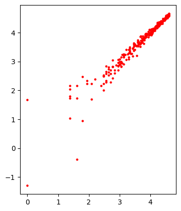
We will be using only a few data points for the model because as the data points and the chain size increase the execution time also increases. Before that, I need to build a function that can apply log on the data and compute the probability accordingly. 

from scipy.stats import norm
logX = np.log(X)
logY = np.log(y)
 
def getLogLike(param):  
    mean = param[0] + param[1] * logX    
    logProbDensities = norm.logpdf(logY, loc = mean, scale = np.exp(param[2])) 
    return np.sum(logProbDensities)

Building the ParaMonte model

para = pm.ParaDRAM()
para.spec.overwriteRequested = True 
para.spec.outputFileName = "./regression_powerlaw" 
para.spec.randomSeed = 100 
para.spec.variableNameList = ["intercept", "slope", "logSigma"]
para.spec.chainSize = 1000 
para.runSampler( ndim = 3 
               , getLogFunc = getLogLike 
               )

• overwriteRequested will overwrite the previously saved result so that it doesn’t interrupt the process of chain creation.
• The report file for samples, chain created and other reports could be saved using ‘outputFileName’.
• For specifying the number of chains to be created using ‘chainsSize’.

After defining all the above parameters, build the sampler and specify the number of parameters in ‘ndim’.

Let’s visualize the chain and the samples created by the sampler.

chain.plot.scatter( ycolumns = "AdaptationMeasure"
                  , ccolumns = [] 
                  )
chain.plot.scatter.currentFig.axes.set_ylim([1.e-5,1])
chain.plot.scatter.currentFig.axes.set_yscale("log")

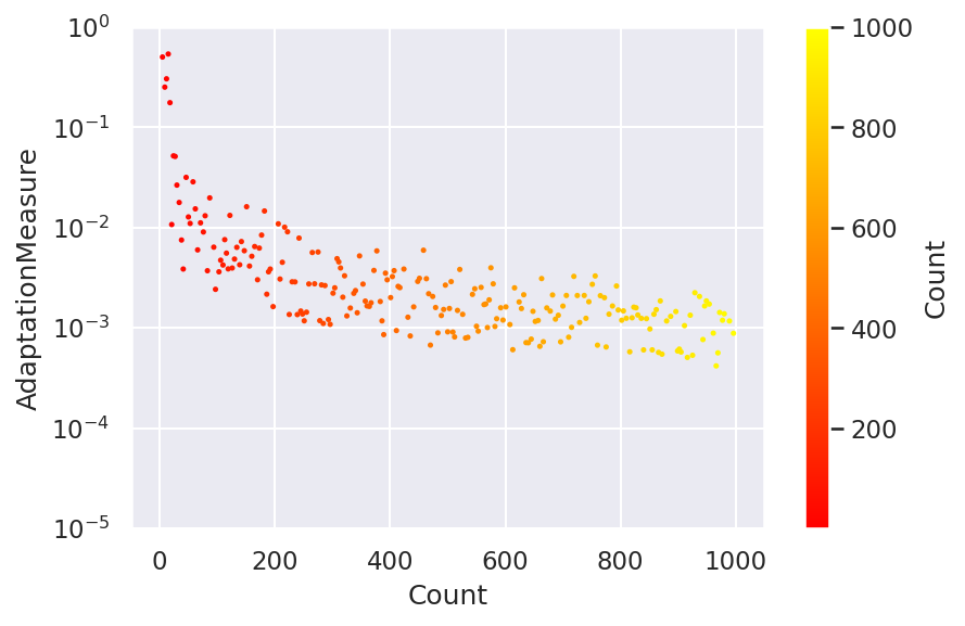
A total of 1000 chains are created as visualized in the above plot with their adaptation score. 

sample = para.readSample(renabled = True)[0]
for colname in sample.df.columns:
    sample.plot.line.ycolumns = colname
    sample.plot.line()
    sample.plot.line.currentFig.axes.set_xlabel("MCMC Count")
    sample.plot.line.currentFig.axes.set_ylabel(colname)
    sample.plot.line.savefig( fname = "/traceplot_" + colname )
 
 
for colname in sample.df.columns:
    sample.plot.histplot(xcolumns = colname)
    sample.plot.histplot.currentFig.axes.set_xlabel(colname)
    sample.plot.histplot.currentFig.axes.set_ylabel("MCMC Count")
    sample.plot.histplot.savefig( fname = "/histogram_" + colname )

As we have taken three variables intercept, slope, and logSigma so there are three different samples. Let’s visualize the distribution of these samples.

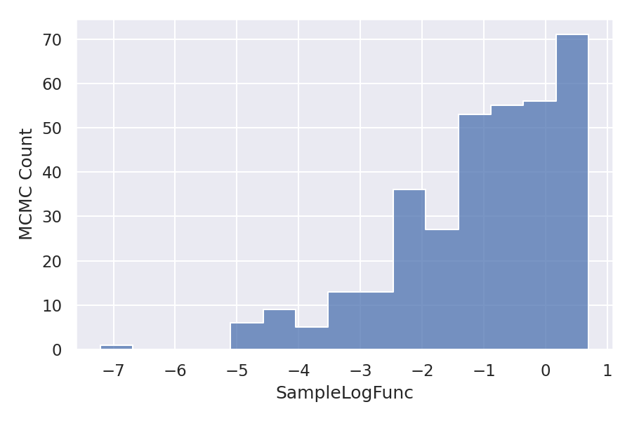
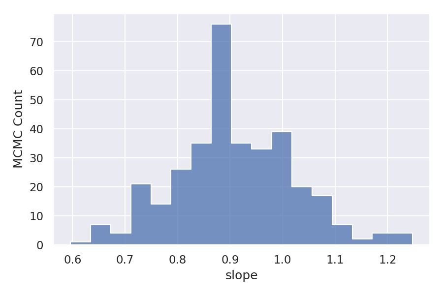
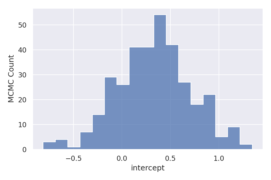
As we can observe the distribution is almost normal for all the variables. But the Log function distribution is skewed to the right. Let’s see how this is affecting the linear relationship between the dependent variable and independent variable.

values = np.linspace(0,100,101)
yvalues = np.exp(sample.df["intercept"].mean()) * xvalues ** sample.df["slope"].mean()
 
fig = plt.figure(figsize = (4.5,4), dpi = 100)
ax = fig.add_subplot(1,1,1)
 
ax.plot(xvalues, yvalues, "b")
ax.scatter(X, y, color = "red", s = 5)

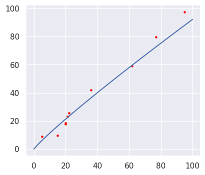
The expected best-fit line, the slope and the intercept learned by the ParaMonte model are shown in the above plot and it can be seen that the relationship line is almost linear. It could be perfectly linear if the skew in the data would be mitigated. As a result, there are many possible regression lines corresponding to each parameter set in the output file, although each one has a different chance of being correct. We can visualize them together to understand the level of uncertainty in our best-fit regression.

values = np.linspace(0,100,101)
 
fig = plt.figure(figsize = (4.5,4), dpi = 100)
ax = fig.add_subplot(1,1,1)
 
 
first = 0
last = 300
slopes = sample.df["slope"].values[first:last]
intercepts = sample.df["intercept"].values[first:last]
 
for slope, intercept in zip(slopes, intercepts):
    yvalues = np.exp(intercept) * xvalues ** slope
    ax.plot( xvalues
           , yvalues
           , "black" 
           , alpha = 0.04 
           )
 
ax.scatter( X, y
          , color = "red"
          , s = 5
          , zorder = 100000
          )

This is only the first set of samples similarly we can visualize the other set of samples.

Final Verdict

ParaMonte is a great package with a parallel implementation of the Monte Carlo Markov Chain which makes the processing time reduced and helps to analyze the data more thoroughly. With a hands-on implementation of this concept, we could do Bayesian data analysis and visualization with ParaMonte.

References

• Link to the above code
• ParaMonte GitHub Repository
• Documentation on ParaMonte