

There are many ways that a system or machine can be taught to ‘learn’ and derive meaning from data. Machine learning is a branch of computer science that focuses on using data and algorithms to make machines intelligent and make the machine simulate how humans learn and how a human brain works, gradually improving its accuracy to provide more efficient results. Machine learning is more dependent on human intervention to learn. Therefore, it requires determining the set of features to understand the differences between data inputs and requires more structured data to learn. Machine learning algorithms are typically used to make a prediction or classification. Then, depending on the input data, which can be labelled or unlabeled, the algorithm will produce an estimate about a pattern present in the data.
Unsupervised learning is one of the ways that a machine learning algorithm learns about data. Unsupervised learning consists of unlabelled data that the algorithm has to try and make sense of independently.
The goal of unsupervised learning is to let the machine learn without any assistance or prompts. It should also learn to adjust the results and groupings and explore more suitable outcomes. It is allowing the machine to understand the data and process it to how it sees fit. According to its similarities, the machine groups the entities together, finding hidden structures and patterns from the unlabelled data.
The data collected and received often don’t come with labels, so using unsupervised learning saves the data scientist from labelling everything, which can be time-consuming and often tedious. Unsupervised learning algorithms also allow obtaining solutions for more complex processing tasks. Having no label means that complicated relationships and clusters of data can be mapped. Using the unsupervised learning method, generative models can be created.
Generative models are models that use an Unsupervised Learning approach, where it uses only the input variables to train the model and recognizes patterns variables to generate an output based on the training data. Generative models can generate new examples from the samples that are similar to other examples present in the data but are indistinguishable as well. The most common example of a generative model can be a Naive Bayes Classifier, often used as a discriminative model. Other examples of generative models include the Gaussian Mixture Model and a modern example that is General Adversarial Networks.
What Are Generative Adversarial Networks?
Generative adversarial networks, also known as GANs is an algorithmic architecture that uses two neural networks, set one against the other and thus the name “adversarial” to generate newly synthesized instances of data that can pass for real data. GANs are used widely in the field of image generation, video generation and voice generation. Ian Goodfellow introduced GANs and other fellow researchers, presented as a paper published at the University of Montreal in 2014. GANs and adversarial training have been referred to as one of the most interesting ideas in the last ten years in ML. GANs’ potential for both being a boon and a bane is huge because they can learn to mimic any distribution of and from the data. GANs can be taught to automatically create many things such as images, music, speech, or prose.
GANs consist of two parts: a generator, which can be described as a neural network that helps generate new data instances, while the other part, known as the discriminator, evaluates them for authenticity. The discriminator decides whether or not each instance of data that it reviews belong to the actual training dataset. The discriminator also penalizes the generator for producing implausible results. It can also be described as adversarial, where the generator tries to trick the discriminator by generating data similar to those present in the training set. The Discriminator tries to identify the fake data from real data, and they both work simultaneously to learn and train complex data such as audio, video or image files.
Here is a pictorial representation of the whole GAN architecture :
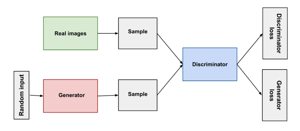
The steps a GAN takes can be summarized as follows :
- A generator takes in a set of random numbers and returns an image.
- This generated image is then fed into the discriminator alongside a stream of images taken from the actual dataset.
- The discriminator compares both the real and fake images and returns probabilities, a number between 0 and 1, where 1 represents a prediction of it being authentic and 0 represents fake.
About the feedback loop:
- The discriminator is always in a feedback loop, providing the ground truth of the images, which we know.
- The generator also stays in a feedback loop with the discriminator.
GANs have come across as an exciting and rapidly changing field, delivering on the promise of generative models’ ability to generate realistic examples across a wide range of problem domains, most notably in the image to image translation tasks such as translation of photos as summer to winter or day to night, and in generating photorealistic photos of objects, scenes, and people, so close to perfection that even humans cannot tell are fake with their naked eye!
Getting Started
This article will implement a GAN model from scratch and see how its different components, such as the generator and discriminator, work in detail using Keras and Tensorflow. We will implement this on the MNIST dataset for ease of understanding and lesser complexity and generate an animated file representing all the image processing steps as they happened in real-time. The following implementation is partially inspired by a video tutorial, whose link can be found here.
Loading The Dataset
Our first step will be to load the MNIST dataset; the following code can be executed to do so
 # loading the mnist dataset
 from tensorflow.keras.datasets.mnist import load_data
Next up, we will be loading the images from the MNIST dataset to the model’s memory and printing train and text shape.
 # load the images into memory
 (trainX, trainy), (testX, testy) = load_data()
 # summarize the shape of the dataset
 print('Train', trainX.shape, trainy.shape)
 print('Test', testX.shape, testy.shape)
Output :
 Train (60000, 28, 28) (60000,)
 Test (10000, 28, 28) (10000,)
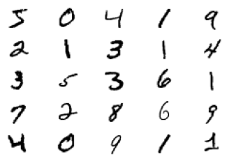
Plotting the images in a 5 row and 5 column order to check the images from the dataset.
 #plot of 25 images from the MNIST training dataset, arranged in a 5×5 square.
 from tensorflow.keras.datasets.mnist import load_data
 from matplotlib import pyplot
 # load the images into memory
 (trainX, trainy), (testX, testy) = load_data()
 # plot images from the training dataset
 for i in range(25):
   # define subplot
   pyplot.subplot(5, 5, 1 + i)
   # turn off axis
   pyplot.axis('off')
   # plot raw pixel data
   pyplot.imshow(trainX[i], cmap='gray_r')
 pyplot.show()
Output :
Installing Dependencies
Installing the further dependencies for our model being created. We are using the imageio library here, which will provide an easy interface to read and write image data and help process an animated image.
 import glob
 import imageio
 import matplotlib.pyplot as plt
 import numpy as np
 import os
 import PIL
 from tensorflow.keras import layers
 import time
 import tensorflow as tf
 from IPython import display
Training the Model
We will further be creating and training the generator and the discriminator. Finally, the generator will generate Unique handwritten digits resembling the MNIST data.
 #setting the training space
 (trn_imag, trn_labl), (_, _) = tf.keras.datasets.mnist.load_data()
 trn_imag = trn_imag.reshape(trn_imag.shape[0], 28, 28, 1).astype('float32')
 trn_imag = (trn_imag - 127.5) / 127.5  # Normalize the images to [-1, 1]
 #setting the buffer and batch size
 BUFFER_SIZE = 60000
 BATCH_SIZE = 256
 # Batch and shuffle the data
 trn_data = tf.data.Dataset.from_tensor_slices(trn_imag).shuffle(BUFFER_SIZE).batch(BATCH_SIZE)
For our generator, we are using tf.keras.layers.Conv2DTranspose (upsampling) layers to produce an image from random noise.
 def genG_model():
     modelG = tf.keras.Sequential()
     modelG.add(layers.Dense(7*7*256, use_bias=False, input_shape=(100,)))
     modelG.add(layers.BatchNormalization())
     modelG.add(layers.LeakyReLU())
     modelG.add(layers.Reshape((7, 7, 256)))
     assert modelG.output_shape == (None, 7, 7, 256)  # Note: None is the batch size
     modelG.add(layers.Conv2DTranspose(128, (5, 5), strides=(1, 1), padding='same', use_bias=False))
     assert modelG.output_shape == (None, 7, 7, 128)
     modelG.add(layers.BatchNormalization())
     modelG.add(layers.LeakyReLU())
    # upsample to 14x14
     modelG.add(layers.Conv2DTranspose(64, (5, 5), strides=(2, 2), padding='same', use_bias=False))
     assert modelG.output_shape == (None, 14, 14, 64)
     modelG.add(layers.BatchNormalization())
     modelG.add(layers.LeakyReLU())
     # upsample to 28x28
     modelG.add(layers.Conv2DTranspose(1, (5, 5), strides=(2, 2), padding='same', use_bias=False, activation='tanh'))
     assert modelG.output_shape == (None, 28, 28, 1)
     return modelG
Using the untrained (for now) generator to create an image.
 # sample image generated by the the generator
 genG = genG_model()
 noise = tf.random.normal([1, 100]) #latent space
 generated_image = genG(noise, training=False)
 plt.imshow(generated_image[0, :, :, 0], cmap='gray')
Output :

Creating the Discriminator
 # Input to discriminator = 28*28*1   grayscale image
 # Output  binary prediction (image is real (class=1) or fake (class=0))
 # no pooling layers
 # single node in the output layer with the sigmoid activation function to predict whether the input sample is real or fake.
 # Downsampling from 28×28 to 14×14, then to 7×7, before the model makes an output prediction
 def make_discriminator_model():
     modelD = tf.keras.Sequential()
     modelD.add(layers.Conv2D(64, (5, 5), strides=(2, 2), padding='same',input_shape=[28, 28, 1])) #2×2 stride to downsample
     modelD.add(layers.LeakyReLU())
     modelD.add(layers.Dropout(0.3))
     modelD.add(layers.Conv2D(128, (5, 5), strides=(2, 2), padding='same')) #downsampling  2×2 stride to downsample
     modelD.add(layers.LeakyReLU())
     modelD.add(layers.Dropout(0.3))
     modelD.add(layers.Flatten())  # classifier real (class=1) or fake (class=0))
     modelD.add(layers.Dense(1, activation='sigmoid'))
     return modelD
     model.add(layers.Flatten())  # classifier real (class=1) or fake (class=0))
     model.add(layers.Dense(1, activation='sigmoid'))
     return model
Using the discriminator function to classify the generated images and generate classification scores.
 discriM = make_discriminator_model()
 decision = discriM(generated_image)
 print (decision)
Output :
tf.Tensor([[0.50052196]], shape=(1, 1), dtype=float32)
Defining the loss and optimizers,
 # This method returns a helper function to compute cross entropy loss
 cross_entropy = tf.keras.losses.BinaryCrossentropy(from_logits=True)
Setting the Discriminator loss to quantify how well the discriminator is able to distinguish the generated images.
 def discriM_loss(real_output, fake_output):
     real_loss = cross_entropy(tf.ones_like(real_output), real_output)
     fake_loss = cross_entropy(tf.zeros_like(fake_output), fake_output)
     total_loss = real_loss + fake_loss
     return total_loss
Setting Generator loss, which will tell us how well it was able to trick the discriminator. Intuitively, if the generator performs well, the discriminator will classify the fake images as real (or 1). Here, compare the discriminator’s decisions on the generated images to an array of 1s.
 def generator_loss(fake_output):
     return cross_entropy(tf.ones_like(fake_output), fake_output)
 Setting the discriminator and the generator optimizers,
 genG_optimizer = tf.keras.optimizers.Adam(1e-4)
 discriM_optimizer = tf.keras.optimizers.Adam(1e-4)
Creating a function to save and restore the models, which can be helpful in case a long-running training task is interrupted.
 checkpoint_dir = './training_checkpoints'
 checkpoint_prefix = os.path.join(checkpoint_dir, "ckpt")
 checkpoint = tf.train.Checkpoint(genG_optimizer=genG_optimizer,
                                  discriM_optimizer=discriM_optimizer,
                                  genG=genG,
                                  discriM=discriM)
Defining the training loop,
 #defining the number of epochs to train for
 EPOCHS = 50
 noise_dim = 100
 num_examples_to_generate = 16
 # You will reuse this seed overtime (so it's easier)
 # to visualize progress in the animated GIF)
 seed = tf.random.normal([num_examples_to_generate, noise_dim])
The training loop begins with the generator receiving a random image as input. The discriminator is then used to classify results from the training set and results produced by the generator. Finally, the loss is calculated for each of these models, and the gradients are used to update the generator and discriminator.
 def trn_img(images):
     noise = tf.random.normal([BATCH_SIZE, noise_dim])
     with tf.GradientTape() as gen_tape, tf.GradientTape() as disc_tape:
       generated_images = genG(noise, training=True)
       real_output = discriM(images, training=True)
       fake_output = discriM(generated_images, training=True)
       gen_loss = genG_loss(fake_output)
       disc_loss = discriM_loss(real_output, fake_output)
     grad_genG = gen_tape.gradient(gen_loss, genG.trainable_variables)
     grad_discriM = disc_tape.gradient(disc_loss, discriM.trainable_variables)
     genG_optimizer.apply_gradients(zip(gradients_of_generator, genG.trainable_variables))
     discriM_optimizer.apply_gradients(zip(gradients_of_discriminator, discriM.trainable_variables))
 def train(dataset, epochs):
   for epoch in range(epochs):
     start = time.time()
     for image_batch in dataset:
       trn_img(image_batch)
     # Produce images for the GIF as you go
     display.clear_output(wait=True)
     sv_img(genG,
                              epoch + 1,
                              seed)
     # Save the model every 15 epochs
     if (epoch + 1) % 15 == 0:
       checkpoint.save(file_prefix = checkpoint_prefix)
     print ('Time for epoch {} is {} sec'.format(epoch + 1, time.time()-start))
   # Generate after the final epoch
   display.clear_output(wait=True)
   sv_img(genG,
                            epochs,
                            seed)
Generate and save images :
 def sv_img(model, epoch, test_input):
   # Notice `training` is set to False.
   # This is so all layers run in inference mode (batchnorm).
   predictions = model(test_input, training=False)
   fig = plt.figure(figsize=(4, 4))
   for i in range(predictions.shape[0]):
       plt.subplot(4, 4, i+1)
       plt.imshow(predictions[i, :, :, 0] * 127.5 + 127.5, cmap='gray')
       plt.axis('off')
   plt.savefig('image_at_epoch_{:04d}.png'.format(epoch))
   plt.show()
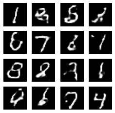
Using the train() method defined above we can train the generator and discriminator simultaneously. Note, training GANs can be tricky. At the beginning of the training, the generated images will look like random noise. As training progresses, the generated digits will look increasingly real. After about 50 epochs, they resemble MNIST digits.
train(train_dataset, EPOCHS)
 # Display a single image using the epoch number
 def display_image(epoch_no):
   return PIL.Image.open('image_at_epoch_{:04d}.png'.format(epoch_no))
 display_image(EPOCHS)
 #create an animated visual which shows changes and training
 !pip install git+https://github.com/tensorflow/docs
 import tensorflow_docs.vis.embed as embed
 embed.embed_file(anim_file)
EndNotes
Through this article, we tried to understand what GAN is and explored its main architectural components. We also created a hands-on GAN model to know how the generator and discriminator in GAN works. I would recommend building more complex models and exploring GAN’s further qualities. The colab notebook for the above implementation can be found using the link here.