Graph neural networks are one of the most emerging techniques in the field of machine learning and deep learning. In many of the research works, we can see the success of these networks in the context of results and speed. One of the major reasons behind the success of graph neural networks is that they use graph data for modelling and graph data can consist of the structural relationship between the entities of the dataset. In this article, we are going to learn how to build and perform modelling with graph neural networks by building and implementing them from scratch. The major points to be covered in this article are listed below.

Table of contents

1. What is a graph neural network? 
2. Understanding the data
   1. Downloading dataset
   2. Visualizing data
   3. Making graph data
3. graph neural network implementation 
   1. Graph layer
   2. Graph neural node classifier 
4. Fitting model
   1. Instantiating GNN model
   2. Defining training data
   3. Training model
   4. Visualizing the results

Let’s begin with understanding what a graph neural network is.

What is a graph neural network? 

In one of our articles, we have discussed that neural networks that can operate on the graph data can be considered graph neural networks. Using graph data any neural network is required to perform tasks using the vertices or nodes of the data. Let’s say we are performing any classification task using any GNN then the network is required to classify the vertices or nodes of the graph data. In graph data, nodes should be presented with their labels so that every node can be classified by their labels according to the neural networks. 

Since in most of the datasets we find that structural relationship between the entities of data we can use the graph neural networks in place of other ML algorithms and can utilize the benefits of using graph data in modelling. The benefits of graph data can be found here.

In this article, we are going to implement a convolutional graph neural network using the Keras and TensorFlow libraries. In this implementation, we will try to use the graph neural network for a node prediction task.

Understanding the data

Using a graph neural network requires graph data. In this article, we are using the Cora dataset. This data set includes 2708 scientific papers that are already classified in 7 classes with 5429 links. Let’s start implementing graph neural network modelling with downloading datasets.

Downloading dataset 

import os
from tensorflow import keras
zip_file = keras.utils.get_file(
    fname="cora.tgz",
    origin="https://linqs-data.soe.ucsc.edu/public/lbc/cora.tgz",
    extract=True,
)
data_dir = os.path.join(os.path.dirname(zip_file), "cora")

Output:

Since the dataset includes two files 

1. cora.cites: Includes the citation records
2. cora.content: Includes the paper content records

 We can see in the output we have two download records.

Now we are required to convert the citation data into a data frame.

import pandas as pd
citations_data = pd.read_csv(
    os.path.join(data_dir, "cora.cites"),
    sep="\t",
    header=None,
    names=["target", "source"],
)

Describing the dataset as,

citations_data.describe()

Output:

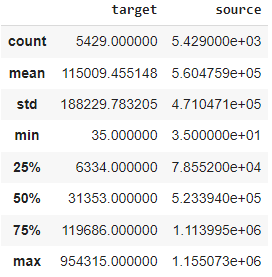
In the description of the data, we can see that the data frame has two variables target and source and the count of the total values are 5429. Let’s convert the core content into a data frame.

column_names = ["paper_id"] + [f"term_{idx}" for idx in range(1433)] + ["subject"]
papers_data = pd.read_csv(
    os.path.join(data_dir, "cora.content"), sep="\t", header=None, names=column_names,
)

Describing the papers data as,

print("Papers shape:", papers_data.shape)
papers_data.head()

Output:

In the output, we can see that this data has 2708 rows and 1435 columns in it with the subject name. Now we are required to provide label encoding to paper ids and subject columns.

class_values = sorted(papers_data["subject"].unique())
class_idc = {name: id for id, name in enumerate(class_values)}
paper_idc = {name: idx for idx, name in enumerate(sorted(papers_data["paper_id"].unique()))}
 
papers_data["paper_id"] = papers_data["paper_id"].apply(lambda name: paper_idc[name])
citations_data["source"] = citations_data["source"].apply(lambda name: paper_idc[name])
citations_data["target"] = citations_data["target"].apply(lambda name: paper_idc[name])
papers_data["subject"] = papers_data["subject"].apply(lambda value: class_idc[value]

Visualizing data

Let’s visualize the graph data using the following lines of codes. 

import networkx as nx
import matplotlib.pyplot as plt
plt.figure(figsize=(10, 10))
colors = papers_data["subject"].tolist()
cora_graph = nx.from_pandas_edgelist(citations_data.sample(n=1500))
subjects = list(papers_data[papers_data["paper_id"].isin(list(cora_graph.nodes))]["subject"])
nx.draw_spring(cora_graph, node_size=15, node_color=subjects)

Output:

In the output, we can see that node is a representation of the graph and the colours of the nodes represent different subjects in the data. As we have discussed that graph neural networks work on the graph data, we are required to convert these data frames into graph data. 

Making graph data

In this section of the article, we will see how we can convert the data frame into graph data. Here we will see a basic approach to making graph data. A basic graph data can consist of the following elements:

1. Node features: This element represents the num of nodes and num of features in an array. The dataset we are using in this article has paper information that can be used as the nodes and the node_features are the word-presence binary vectors of each paper.
2. Edges: This is a sparse matrix of links between the nodes that represent the number of edges in both dimensions. In our data set, links are the paper citations.
3. Edge weights: This is an optional element that is an array. Values under this array represent the number of edges which is a quantification between nodes. Let’s see how we can make them.

import tensorflow as tf
feature_names = set(papers_data.columns) - {"paper_id", "subject"}
feature_names

Output:

• Edges 

edges = citations_data[["source", "target"]].to_numpy().T
print("Edges shape:", edges.shape)

Output:

• Node features 

node_features = tf.cast(
    papers_data.sort_values("paper_id")[feature_names].to_numpy(), dtype=tf.dtypes.float32
)
print("Nodes shape:", node_features.shape)

Output:

• Edge weight

edge_weights = tf.ones(shape=edges.shape[1])
print("Edges_weights shape:", edge_weights.shape)

Output:

Now we can create a graph info tuple that consists of the above-given elements.

graph_info = (node_features, edges, edge_weights)

Now we are ready to train a graph neural network using the above-made graph data with essential elements.

Implementing the graph neural network

As discussed above in this section we will be building a network that can work with the graph data. For this, we are required to make a layer that can work on the graph data.

Graph layer  

In this section of the article, we are going to discuss the tasks which a basic graph layer needs to perform. Since the size of the code is big we are not pushing it here but we will be discussing the task and functionality of the layer. We can find the whole implementation here. Let’s start with the first task.

• This task is about the preparation of input nodes which we have implemented using a feed-forward neural network. That network will produce a message so that input node representations can be processed. The shape of the node representation will be [num_nodes, representation_dim].
• The next task is about the aggregation of the messages provided by the node to its neighbour node using the edge weights. In mathematics, we are using permutation invariant pooling operations here. These operations create a single aggregated message for each node. The shape of the aggregated messages will be [num_nodes, representation_dim].
• The next task is about the production of a new state of the node representations. In this task, we are combining the node representation and aggregated messages. Basically, if the combination is of GRU type then node representations and aggregated messages can be stacked to create a sequence and processed by a GRU layer. 

For performing these tasks, we have created a graph convolutional layer as a Keras layer consisting of prepare, aggregate, and update functions. 

Graph neural node classifier 

After making the layer we are required to make a graph neural node classifier. This classifier can follow the following processes:

• Preprocessing of the node features to generate the node representation.
• Applying graph layers.
• Post-processing of the node representation to generate final node representations.
• Using a softmax layer to produce the predictions based on the node representation.

Since the code of this section is also big, we are pushing them here. We can find the implementation here. In the codes, we have applied two graph convolutional layers for modelling the graph data.

Fitting model

Let’s fit the graph neural network now.

Instantiating GNN model

hidden_units = [32, 32]
learning_rate = 0.01
dropout_rate = 0.5
num_epochs = 300
batch_size = 256
gnn_model = GNNNodeClassifier(
    graph_info=graph_info,
    num_classes=num_classes,
    hidden_units=hidden_units,
    dropout_rate=dropout_rate,
    name="gnn_model",
)
gnn_model.summary()

Output:

Here we have instantiated the model.

Defining training data 

x_train = train_data.paper_id.to_numpy()
y_train = train_data["subject"]

Defining function for compiling and fitting the model

def run_experiment(model, x_train, y_train):
    # Compile the model.
    model.compile(
        optimizer=keras.optimizers.Adam(learning_rate),
        loss=keras.losses.SparseCategoricalCrossentropy(from_logits=True),
        metrics=[keras.metrics.SparseCategoricalAccuracy(name="acc")],
    )
    # Create an early stopping callback.
    early_stopping = keras.callbacks.EarlyStopping(
        monitor="val_acc", patience=50, restore_best_weights=True
    )
    # Fit the model.
    history = model.fit(
        x=x_train,
        y=y_train,
        epochs=num_epochs,
        batch_size=batch_size,
        validation_split=0.15,
        callbacks=[early_stopping],
    )
 
    return history

Training model 

history = run_experiment(gnn_model, x_train, y_train)

 Output:

Visualizing the results 

Loss

fig, ax1 = plt.subplots(1, figsize=(15, 5))
 
ax1.plot(history.history["loss"])
ax1.plot(history.history["val_loss"])
ax1.legend(["train", "test"], loc="upper right")
ax1.set_xlabel("Epochs")
ax1.set_ylabel("Loss")

Output:

Accuracy 

fig, ax2 = plt.subplots(1, figsize=(15, 5))
ax2.plot(history.history["acc"])
ax2.plot(history.history["val_acc"])
ax2.legend(["train", "test"], loc="upper right")
ax2.set_xlabel("Epochs")
ax2.set_ylabel("Accuracy")
plt.show()

Output:

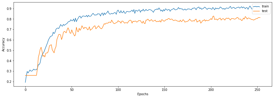
Here in the above output, we can see that the model has performed well. In the accuracy part, we can see that the model has given us accuracy around 90% in training and 80% in testing data.

Final words

In this article, we have seen how we can design data as graph data and how we can implement a graph neural network to work with the graph data. In-depth, we can say that we have implemented a convolutional graph neural network that can also work with graph data with sequential attributes.

Reference

• Link to the above codes
• Graph Neural Networks