For an algorithm to be termed “efficient”, its execution time must be constrained by a polynomial function of the input size. It was realised early on that not all issues could be handled thus rapidly, but it was difficult to determine which ones could and which couldn’t. Some so-called NP-hard issues are thought to be impossible to answer in polynomial time. NP-hard stands for non-deterministic polynomial-time hardness. This article will be focused on understanding some NP-hard problems and trying to solve them with Reinforcement Learning. Following are the topics to be covered.
Table of contents
- Understanding NP Problems
- When a problem is classified as NP-hard?
- Reinforcement learning for solving NP-hard problem
A decision problem has a single boolean output: Yes or No. Let’s understand more about when a decision problem becomes non-deterministic.
Understanding NP Problems
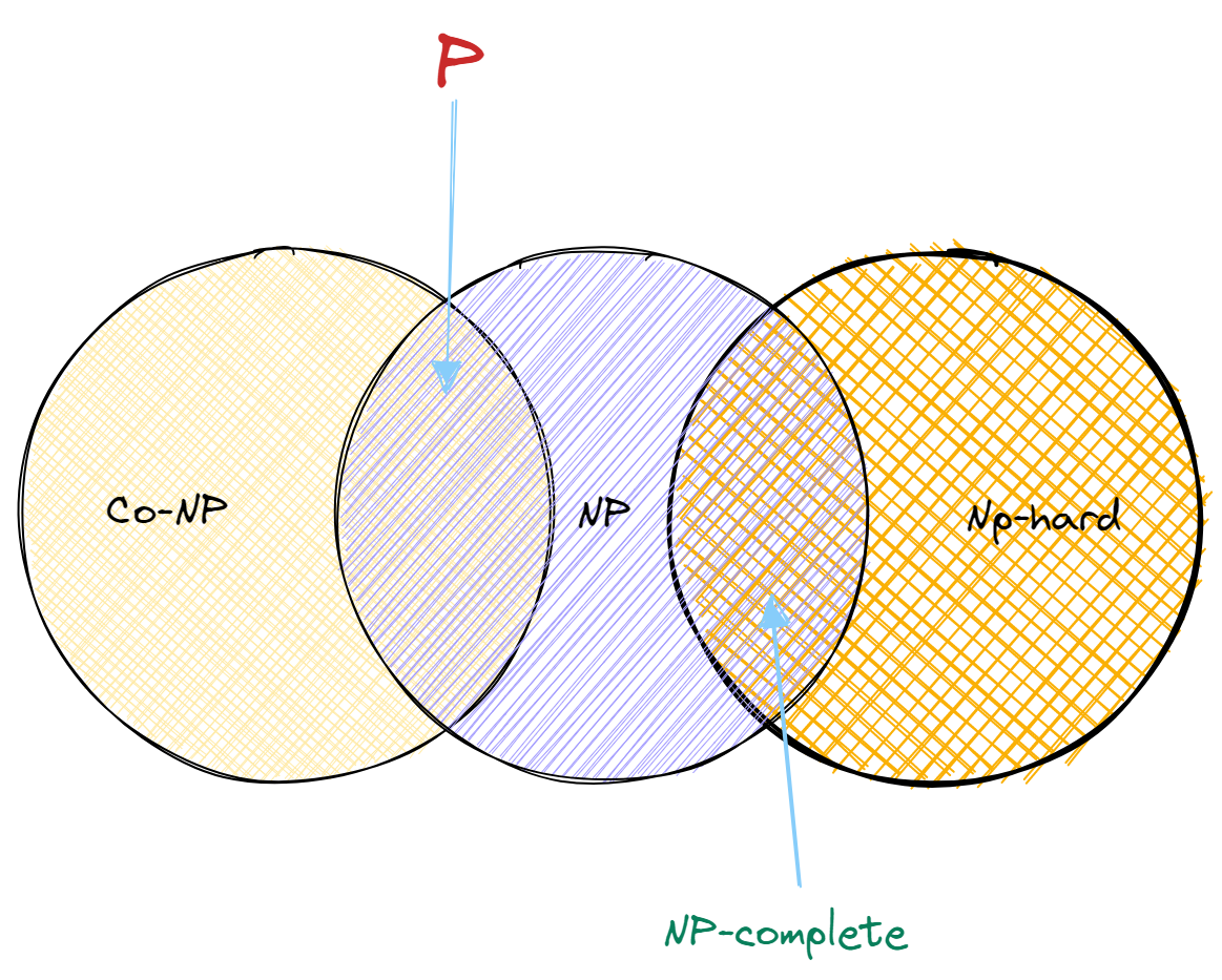
Generally, those sets of decision problems that can be solved under a polynomial-time are categorized as ‘P’. The decision problem that can be proved and verified the answer to the problem is a ‘Yes’ in a polynomial time is classified as NP. NP is intuitively defined as the set of decision problems where it can prove a ‘Yes’.
The circuit satisfiability issue, for example, is in NP. If a given boolean circuit is satisfiable, then every combination of m input values that generate True output is proof that the circuit is satisfiable; the proof may be checked by evaluating the circuit in polynomial time. It is commonly assumed that circuit satisfiability is not in P or co-NP, although no one knows for sure.
If a polynomial-time algorithm for the problem implies a polynomial-time algorithm for every problem in NP, the problem is NP-hard. Intuitively, if one specific NP-hard issue can be solved rapidly, then any problem with an easy-to-understand answer may be addressed using the solution to that one special problem as a subroutine. NP-hard issues are as least as difficult as any other problem in NP.
Finally, a problem is said to be NP-complete if it is both NP-hard and contains an element of NP. Informally, NP-complete issues are the most difficult for NP. A polynomial-time algorithm for only one NP-complete issue implies a polynomial-time algorithm for all NP-complete problems.
Are you looking for a complete repository of Python libraries used in data science, check out here.
When a problem is classified as NP-hard
A reduction argument can be used to demonstrate that any problem is NP-hard. Reducing issue A to another problem B entails explaining an algorithm to solve problem A while assuming that an algorithm to solve problem B already exists.
To demonstrate that your problem is difficult, an efficient method to solve a different problem that is already known to be difficult must be given, utilising a hypothetical efficient programme treating the problem as a black-box subroutine. Proof by contradiction is the core logic.
The reduction indicates that if the first problem were easy, the second problem would be easy as well, which it isn’t. Alternatively, because the previous issue is known to be difficult, the reduction implies that the current problem must likewise be difficult; the hypothetical efficient method does not exist.
For example, a finite set of integers are given and need to find that any non-empty subset of them adds up to zero. To prove that this problem is an NP-hard problem needs to use 3CNF SAT.
- Conjunctive normal form (CNF) boolean formulas are those that are represented as conjunctions (AND) of clauses, each of which is the disjunction (OR) of one or more literals. If each sentence has precisely three different literals, the boolean formula is in 3-conjunctive normal form (3CNF SAT).
The reduction method builds instance sets and targets given a three CNF formula over variables with clauses each having precisely three different literals. Two assumptions must be made to establish that this issue is NP-hard: first, no sentence contains both the variable and its negation, and second, each variable appears in at least one clause. This will be regarded as an NP-hard task.
Reinforcement learning for solving NP-hard problem
Reinforcement learners are taught a series of decisions. In an uncertain, possibly complicated environment, the agent learns to attain a goal. The method uses trial and error to find a solution to the problem. Its objective is to maximise overall return.
The reward policy, which is the training rules, is specified, and the model is given no cues or ideas for how to tackle the problem. It is up to the model to choose how to accomplish the job to maximise the reward, beginning with completely random trials and progressing to complex tactics.
Let’s take a few NP-hard examples and understand the solution to them using Reinforcement Learning.
Capacitated Vehicle Routing Problem
The Vehicle Routing Problem is a combinatorial optimization problem in which the aim is to find the most cost-effective routes for a fleet of vehicles to take to serve a given set of clients. Despite its simplicity, the VRP belongs to the family of NP-hard problems, which are distinguished by their exponentially growing difficulty in finding a solution as the issue grows in size.
To give a few examples of VRP, consider the e-commerce giant Amazon, which delivers 2.5 billion packages per year while constantly attempting to optimise every step of the process, including determining the best route their drivers should take to deliver the parcels on time and at the lowest possible cost. The Uber issue is a variation of the VRP in which the corporation wishes to allocate the best possible routes to drivers to pick up and drop off clients.
The purpose of the CVRP is to serve each customer’s demand with a fleet of homogenous vehicles, all starting from a specific node called the depot and with a defined capacity of carried items. A van will visit each client one at a time, completing their orders and returning to the depot after the entire truckload has been delivered. The cost of travelling between two nodes is just the Euclidean distance between them.

The depot is represented by the squared node, the customers are represented by the circled nodes, and the network is fully linked and undirected. The dotted lines indicate the pathways that were not chosen in the suggested solution. The Euclidean distance between two nodes is the cost associated with each edge. The highlighted pathways reflect a workable solution since all five clients have been visited and the total of the amounts fulfilled in each of the two trips is less than or equal to the delivery vehicle capacity Q. The recommended solution is also optimum in terms of the total distance travelled.
The CVRP may be viewed as a sequential decision-making issue in which the vehicle must select where to go next at each timestep to complete its task of servicing all clients. With this viewpoint, the components characterising the RL issue may be expressed. State, Action and Reward spaces Each customer’s node on the graph is related to their current demand as well as their location. When a vehicle visits a node, whether to meet a client’s demand or to replenish the truck at the depot, the graph can be updated to represent the current condition of the system.
The depot’s location is critical to know, especially when the truck is nearly empty and needs to return to the depot to refill. Depending on the volume of items still in the truck, it may be advantageous to pick a node closer to the depot because the truck will need to get there shortly. As a result, the present load in the vehicle must also be reflected in the state space. The location of each node and the present position of the truck are critical pieces of information to offer to the learning agent for it to grasp the cost of travelling from one node to another.
Finally, the present demand of each client aids in determining which nodes have yet to be visited and are candidates for the truck’s next destination. More information, such as the distance travelled or the prior position can be added to the state space. The more information that may assist the policy’s neural network in making the optimum choice, the better. However, there is a trade-off to consider: if there is too much information, the “curse of dimensionality” will be an issue, and the training will most likely take too long.
The action space is a limited collection of actions that determine which node the vehicle visits next. In principle, the policy might choose any node at any timestep. However, returning to the same node or travelling to the depot while having enough load to serve at least one more client is extremely inefficient. These two tactics would be used to steer the decision-making process.
- When the truck’s current load is insufficient to meet customer demand, the related nodes are masked off during the action selection process to ensure that these nodes are not picked.
- When a client node’s demand is met, it is masked out until the run ends.
This new logic aids the RL algorithm’s exploration phase and applies to all CVRP instances. The problem’s reward signal is comparable to the MIxed integer programming (MIP) formulation: the aim is to identify the cheapest routes travelled by truck, and the purpose of the RL is to maximise the cumulative reward, thus we use the inverse of the total distance travelled.
The RL algorithm is subjected to various issue setups with a fixed set of nodes that are at different places each time. Exposing the learning agent to a large number of cases allows the learned policy to generalise and prevent overfitting to a single CVRP instance. A run begins with all of the customers’ wants unfulfilled and the truck in the depot; the agent then interacts with the environment by visiting nodes until all of the customers’ demands have been met. Only after each episode is the routes chosen evaluated, resulting in the award for this run.
Because the masking approach only allows particular nodes to be picked, the trained policy’s solution is guaranteed to be practical. However, there is no assurance that the proposed solution is optimum; the algorithm learns to reduce the distance travelled but has no idea of the minimum that may be attained; thus the algorithm’s exploration phase could progress towards the ideal solution or become trapped in a local minimum. As a result, the RL technique can only be classed as a heuristic method.
Graph mining
Heterogeneous Information Networks (HINs) can be used to simulate complex interactions in real-world data, such as social networks, biological networks, and knowledge graphs. HINs are typically connected with numerous types of objects/nodes and meta-relationships.

Using the previously illustrated heterogeneous academic network as an example, it has four categories of nodes: papers, authors, institutions, and publication venues, as well as eight types of meta-relationships between these nodes.
Traditional machine learning techniques struggle to model HINs due to their complicated semantics and non-Euclidean nature. Through sequential exploration and exploitation, Deep Reinforcement Learning agents may adaptively create optimal meta-paths for each node in terms of a given goal. This is appealing and feasible for HINs with complicated semantics.
An MDP’s main components are a collection of states, a set of actions, a decision policy, and a reward function. A meta-path is constructed with maximum timesteps that can be characterised as a circular decision-making process that can be treated naturally as an MDP. The initial node’s characteristics as state, and selecting one relation is the first step in expanding the meta-path. Following the expanded meta-path, build appropriate meta-path instances for the algorithm to learn node representations for use in a downstream prediction task to get reward scores. The meta-path design method is formally formulated as follows.
The state space is utilised to aid the decision policy in determining which relation to applying while extending the meta-path. It is critical to record all relevant information in an existing meta-path. As a result, the state is configured to remember all nodes participating in the meta-path.
The action space for a state is comprised of the set of accessible relation types in the HIN as well as the unique action STOP. Beginning with the initial node, the decision strategy predicts the most promising relation for extending the current meta-path to get a higher reward score repeatedly. It may either approach the maximum timestep or discover a node representation that any more relation in the meta-path would impair the performance of node presentations on the downstream job, in which case the decision policy selects the action STOP to complete the path design process.
An MDP’s decision policy seeks to map a state in state space into action in action space. The state space and action space in the meta route design process are continuous space and discrete space, respectively. To estimate the action-value function, a deep neural network is utilised. Furthermore, because every random action is always a positive integer, the DQN Q-network is employed as the decision policy network. As the deep neural network for the Q-network, an MLP is used. The output represents the possibility of extending the meta-path by selecting other relations in the action space.
The reward is an important aspect in directing the RL agent, encouraging it to attain greater and more steady performance. Thus, the reward is defined as an improvement in performance on a certain task relative to previous performances. The objective job is node classification, and the evaluation performance is based on its accuracy on the validation set.
According to the descriptions above, the suggested meta route design process of node at timestep contains three phases:
- Getting the timestep’s state
- Forecasting an action based on the present state to extend the meta-path
- Current state updating
Back-propagation and gradient descent are used to improve the Q-network parameters by minimising the loss function.
Travel Salesman Problem
The travelling salesman problem (TSP) is an algorithmic problem in which the goal is to discover the shortest path between a collection of points and places that must be visited. The cities that a salesman could visit are represented by the points in the problem statement. The objective of the salesman is to minimise both travel expenditures and distance travelled.
The TSP RL solution has an encoder-decoder design. The first city to visit is chosen at random since the trip should be invariant to the initial city. As a result, the solver’s decisions begin at a time step greater than 2. In translation, invariance may be further leveraged by evaluating relative locations of the most recently visited city rather than the original absolute coordinates. The RL solver’s input consists of simply two bits of information.
- The present partial tour information now just requires the relative preprocessed location of the first visited city. Because the most recently visited city is always represented by the origin, it can be omitted.
- The remaining TSP instance information relates to the relative preprocessed locations of the unvisited cities, as well as the first and last visited cities.
The relative preprocessed locations are saved in a matrix, which includes the most recently visited city. Because it represents the labels of the remaining graph nodes on which the tour should be finished.
The model’s encoder is made up of a graph neural network (GNN) that computes an embedding of the relative city locations and a multilayer perceptron (MLP) that computes an embedding of the first visited city. The GNN encapsulates the graph information characterising the remaining TSP issue. It is invariant with regard to the order of its inputs as a GNN, and its outputs are dependent on the graph structure and information (i.e., city positions).
The MLP encodes information about cities visited. Since the independence of the visited cities between the first and last cities (not included) is used. For encoding the locations of the visited cities, the model does not require any sophisticated architecture, such as LSTM. Because just the relative location of the first city is required, a basic MLP suffices.
After computing the embeddings, the probability of choosing the next city to visit is calculated using a conventional attention mechanism with relative location and first city as the keys and queries, respectively. The decoder produces a trainable weight vector. The vector is then transformed into a probability distribution using a softmax transformation.
Conclusion
Reinforcement Learning necessitates a training phase in which the algorithm learns the optimum course of action to take after being exposed to a variety of configurations. Because of its simplicity, just the problem’s rules must be defined, and the algorithm learns how to solve the problem via trial and error. With this article, we have understood NP-hard problems and their solution through Reinforcement Learning.


