In today’s scenario, image processing and computer vision are the subjects of attraction in the data science world. If we consider an image as data, we can extract a lot of information like the objects presented in an image, how many colors, and the pixel configurations of the image. And also, in various cases of machine learning, images take part as an informative member of the process. Many image processing applications in the machine learning field like object detection, face recognition, threat detection, etc. Before going into the modeling part, I recommend working with the editing part of the image. There can be a number of basic operations we can perform in an image. This article is mainly focused on the following processes:
- Image translation
- Parametric transformation
- Image warping
Between all these things, we will also have some basic reading knowledge, displaying and saving the image, and rotating and resizing an image using OpenCV-python.
Implementations with OpenCV
Let’s start with the installation of the OpenCV-Python.
!pip install opencv-python
Output:

As I am using google Colab, it already provides the OpenCV installed in the notebook environment.
Reading the image.
import cv2
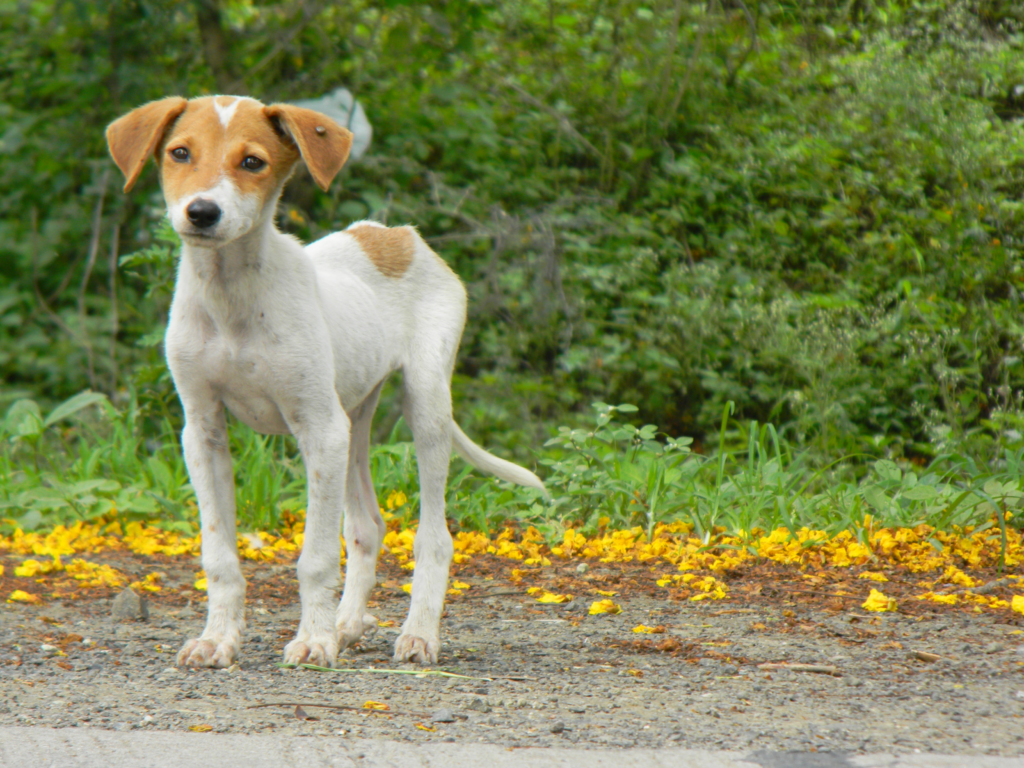
image = cv2.imread('/content/drive/MyDrive/Yugesh/image wraping/DSCN9772.JPG')
(Note – cv2.imshow() is disabled in Colab, because it causes Jupyter sessions
to crash; see https://github.com/jupyter/notebook/issues/3935. As a substitution, consider using from google.colab.patches import cv2_imshow )
Displaying the image:
from google.colab.patches import cv2_imshow
cv2_imshow(image)
cv2.waitKey()
Output:
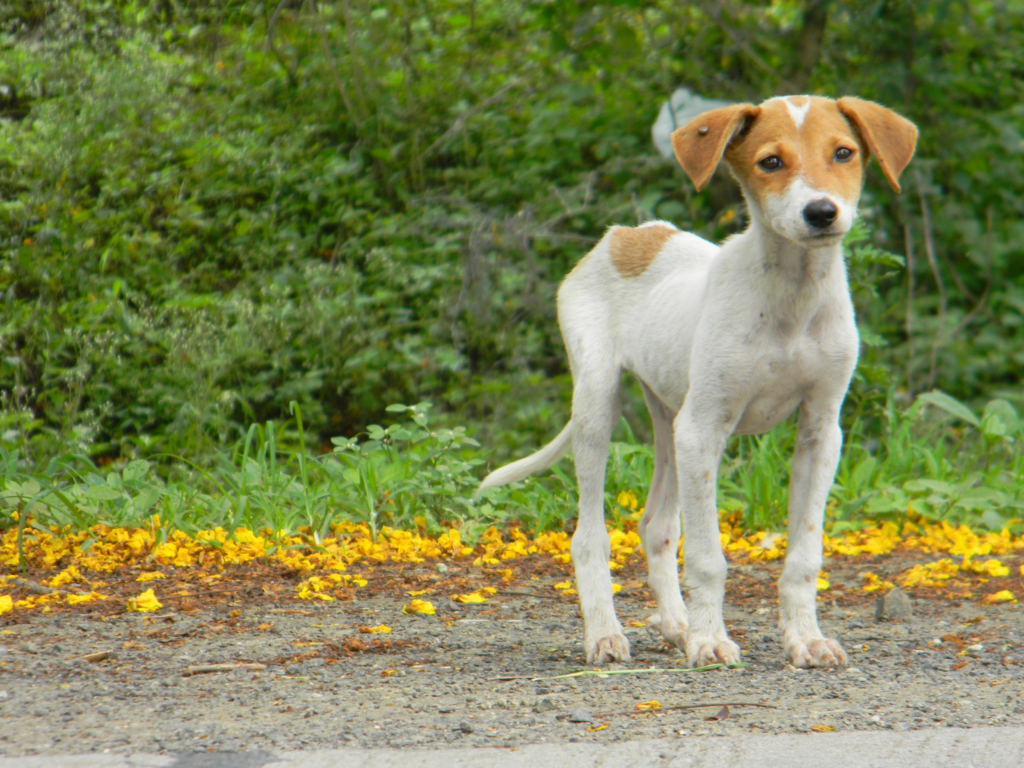
From the above lines of codes, you can read and display whatever image you want.
Checking the data structure:
print(image.shape)
print(image.size)
print(type(image))
Output:

Here we can see the shape and size of the image. Since OpenCV uses a NumPy data structure to store the images, it shows the type of data as numpy.ndarray. We can also change the color space of the image. For example, the image we have read is in BGR color space.
gray = cv2.cvtColor(image, cv2.COLOR_BGR2GRAY)
cv2_imshow(gray)
Output:
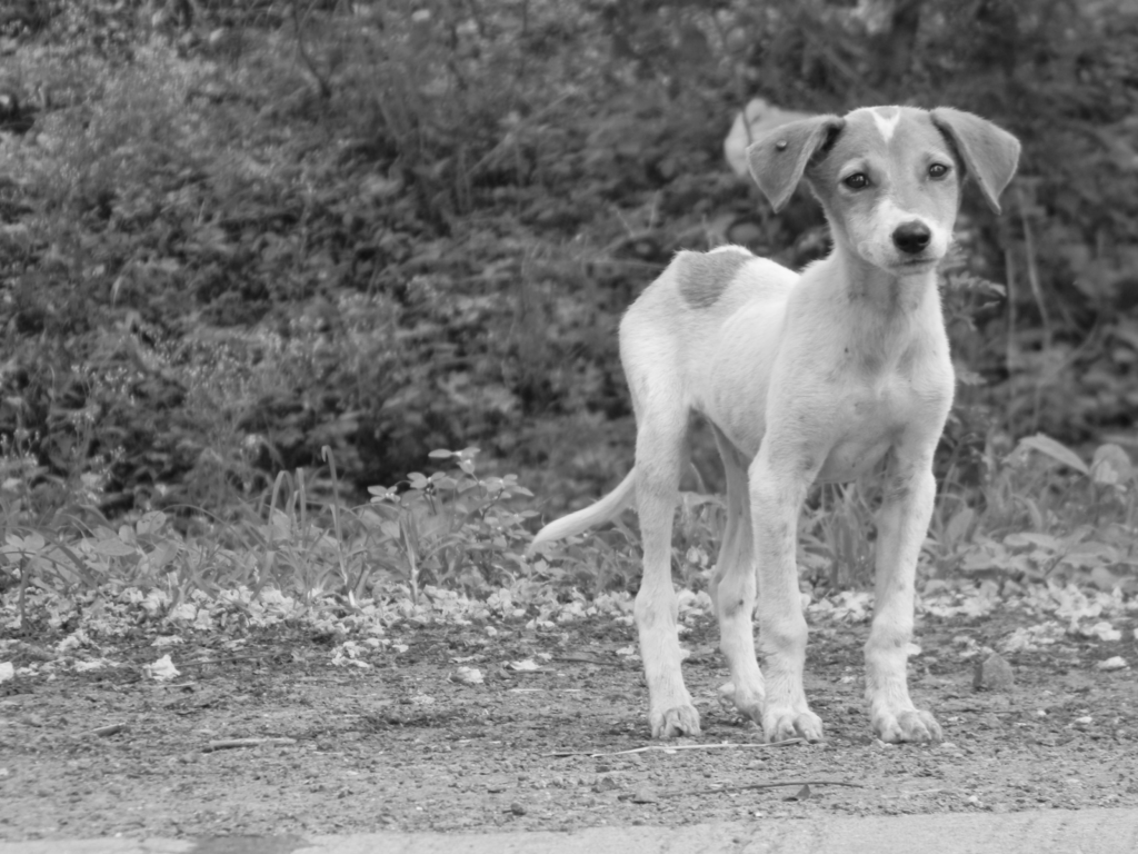
There are various color spaces available in the package. Here we have changed the space using the cv2.COLOR_BGR2GRAY function. Converting the image color space BGR to RGB.
rgb = cv2.cvtColor(image, cv2.COLOR_BGR2RGB)
cv2_imshow(rgb)
Output:
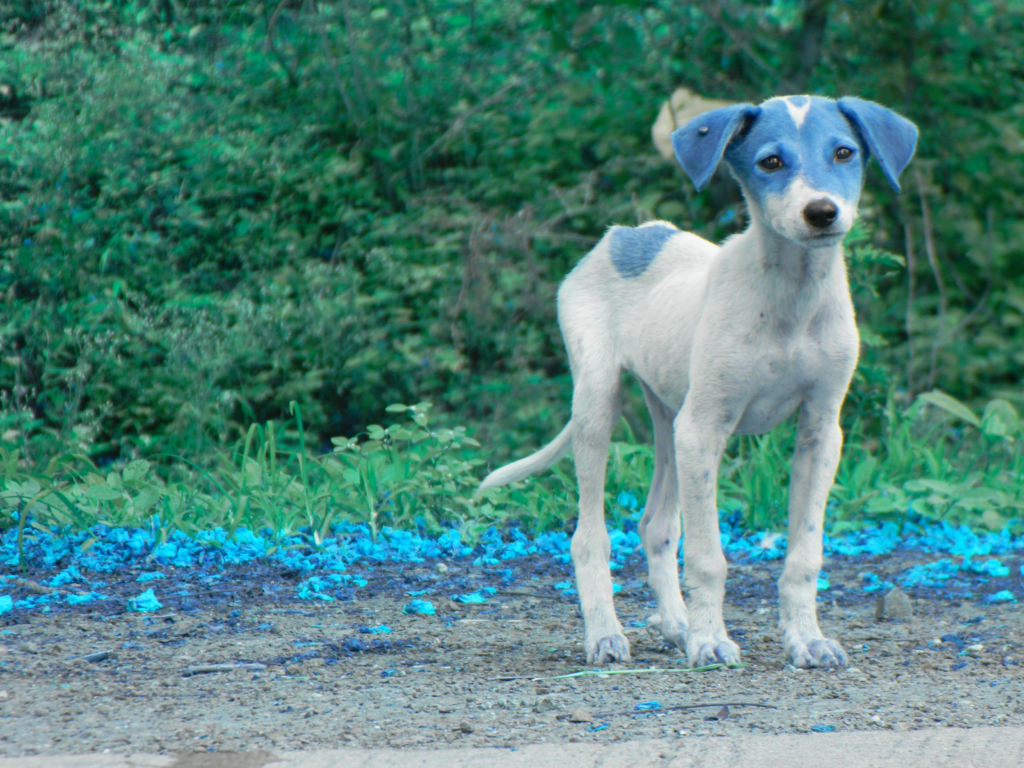
Here we have seen when we read an image using OpenCV by default, its color space is set on the BGR color space and using the function, we can change the colour space.
Saving the image.
cv2.imwrite('/content/drive/MyDrive/Yugesh/image wraping/output.png', rgb, [cv2.IMWRITE_PNG_COMPRESSION])Output:

Here you must be wondering why I used the cv2.IMWRITE_PNG_COMPRESSION function in saving the image. When I imported the image, it was a jpg format photo, and we saved it as a png format image.
In image processing, the color space refers to the space where the patterns of the color are organized in different manners. Combining a color model and a mapping function makes a color space. The color model helps represent the pixel values in tuples, and the mapping function maps the color model to set all colors that can be represented. There are around 190 color spaces present in the OpenCV, out of which we can choose according to the requirements. For more information about the list, you can go through this link.
Next in the article, we will see how we can perform editing in any image structure. The first thing we are performing is called image translation.
Image Translation
In computer vision or image processing, shifting an image into a frame is considered as the image translation.
Let’s see how we can perform that.
num_rows, num_cols = image.shape[:2]
translation_matrix = np.float32([ [1,0,70], [0,1,110] ])
img_translation = cv2.warpAffine(image, translation_matrix, (num_cols, num_rows), cv2.INTER_LINEAR)
Displaying the translated image:
cv2_imshow(img_translation)Output:

Here in the output, we can see that we have shifted the image in the frame. To understand the code part first, we need to go through the warpaffine function. It takes a matrix as a parameter in the matrix we give x = 70, which means we are telling the function to shift the image 70 units on the right side and y= 110, which means we are telling the function to shift the image 110 units downwards.
In the third argument, where we mentioned the num_cols and num_rows, we told the function to crop the image by two units from both x and y sides.
We can also set the image without cropping the image in the middle of the frame.
translation_matrix = np.float32([ [1,0,-30], [0,1,-50] ])
img_translation = cv2.warpAffine(img_translation, translation_matrix, (num_cols + 70 + 30, num_rows + 110 + 50))
cv2_imshow(img_translation)
Output:
Here in the input, we have told the function to shift the image upward and to the left side and added the total value of x and y from the translation matrix in num-row and num_col to avoid the cropping of the image.
Next, in the article, we will see how we can rotate and scale the image.
Image Rotation.
In this section we will try to rotate the image by a certain angle:
img_rotation = cv2.warpAffine(image, cv2.getRotationMatrix2D((num_cols/2, num_rows/2), 30, 0.6), (num_cols, num_rows))Output:

Here in the codes, we have used the getRotationMatrix function to define the parameter required in the warpAffine function to tell the function to make a matrix that can give a required rotation angle( here it is 30 degrees) with shrinkage of the image by 40%.
Image Scaling
This is a commonly used method in the computer vision and image processing area where we try to resize the image according to the requirement. Roughly we perform two things in the image scaling: either we enlarge the image or we shrink the image; in OpenCV, we have function resize; using this, we can perform the scaling of the image.
Shrinking the image:
img_shrinked = cv2.resize(image,(350, 300), interpolation = cv2.INTER_AREA)
cv2_imshow(img_shrinked)
Output:

Enlarge the image size.
img_enlarged = cv2.resize(img_shrinked,None,fx=1.5, fy=1.5, interpolation = cv2.INTER_CUBIC)
cv2_imshow(img_enlarged)
Output:

Here in the code, we resize the image to (350, 300), and after this, we enlarged the shrunk image by a factor of 1.5. We had used INTER_AREA interpolation when we were shrinking the image, and then we used CUBIC interpolation when enlarging the image so that the quality of pixels will not be harmed while resizing.
Image Transformation
In image processing, image transformation can be defined as having control on its dimensional points to edit the images by moving them into three dimensional or two-dimensional space. Next in the article will perform some basic transformations of 2D images. Before going into the implementation of image transformation, let’s see what is euclidean transformation. Euclidean transformation is a type of geometric transformation that causes changes in the dimensions and angles without causing the change in the basic structure-like area. Image Transformation works based on euclidean transformation, where the image can look shifted or rotated, but the structure of pixels and matrix will remain the same.
Roughly we can divide image transformation into two sections:
- Affine transformation.
- Projective transformation.
Affine transformation
As the name suggests in this transformation, preserving parallel relationships is one of the main concepts of this kind of transformation where lines will remain the same. Still, the square can change into a rectangle or parallelogram. It works by preserving the lengths and angles. The following example will give a better view of the Affine transformation where I am implementing it using the getAffineTransformation function.
src_points = np.float32([[0,0], [num_cols-1,0], [0,num_rows-1]])
dst_points = np.float32([[0,0], [int(0.6*(num_cols-1)),0], [int(0.4*(num_cols-1)),num_rows-1]])
matrix = cv2.getAffineTransform(src_points, dst_points)
img_afftran = cv2.warpAffine(image, matrix, (num_cols,num_rows))
Displaying the image and transformed image.
cv2_imshow(image)
cv2_imshow(img_afftran)
Output:

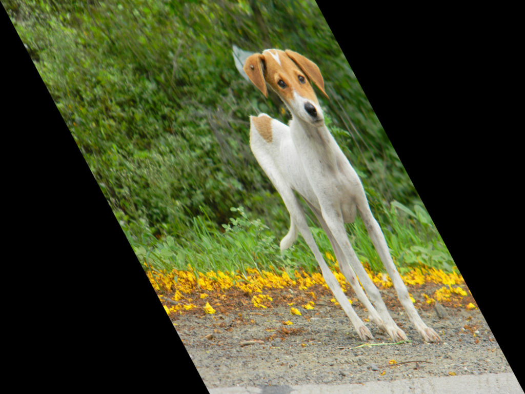
Here we can say how we have changed the image. The image we have used was in the rectangle shape, and after transformation, it became a parallelogram. We included two control points in the affine transform matrix and told the getAffineTransform function to map those points in different places.
We can also make a mirror image of the original image.
src_points = np.float32([[0,0], [num_cols-1,0], [0,num_rows-1]])
dst_points = np.float32([[num_cols-1,0], [0,0], [num_cols-1,num_rows-1]])
matrix = cv2.getAffineTransform(src_points, dst_points)
img_afftran = cv2.warpAffine(image, matrix, (num_cols,num_rows))
cv2_imshow(image)
cv2_imshow(img_afftran)
Output:

The mapping of the points in this transformation will look like the following image.
Where we just selected the outermost points of the image as the control points.
Projective Transformation:
As seen in the Affine transformation, we have less control in shifting the points, but in projective transformation, we have the freedom to move and shift the control points. It works on the projective view option where we see an object from its every plane. For example, a square image on paper from the front side looks like a square, but it will look like a trapezoid from the slight right or left side.
Implementation of the projective transformation will explain it more.
src_points = np.float32([[0,0], [num_cols-1,0], [0,num_rows-1], [num_cols-1,num_rows-1]])
dst_points = np.float32([[0,0], [num_cols-1,0], [int(0.33*num_cols),num_rows-1], [int(0.66*num_cols),num_rows-1]])
projective_matrix = cv2.getPerspectiveTransform(src_points, dst_points)
img_protran = cv2.warpPerspective(image, projective_matrix, (num_cols,num_rows))
Displaying the image:


Let’s imagine you see the image(not transformed) from the upside of the screen; the normal image looks like this. This editing of the image mostly helps in the object detection program. By projective view, we extract most of the features available in the image. In this transformation, we have changed a rectangular into a trapezoid. We have freedom here to shift our angles and the points; we can even make the image look like a triangle.
Image Wrapping
We have seen how the transformation works, but what if we need to randomly put these effects in a single picture, or do we just need to shift the control points in the space randomly? Then we require more control over the movements. We have seen that projective transformation increased the level of control, but still, some restrictions were there. In projective transformation, we were working with dimensions, lengths and angles. Now we will see how we can work on randomly selected points from the image to change the surface of the image, which will put the wave-like edits in the image.
import math
rows, cols = image.shape[:2]

# Vertical wave

img_output = np.zeros(img_afftran.shape, dtype=image.dtype)
for i in range(rows):
    for j in range(cols):
        offset_x = int(25.0 * math.sin(2 * 3.14 * i / 180))
        offset_y = 0
        if j+offset_x < rows:
            img_output[i,j] = img_afftran[i,(j+offset_x)%cols]
        else:
            img_output[i,j] = 0
Displaying the image.
cv2_imshow(img_output)
Output:

Here we have pushed a sine wave into the image, vertically moving on the surface of the image. This is how we can perform the image wrapping. Using a cos wave, we can also put a horizontal wave into the image.
Here in the article, we have seen how we can perform basic modifications in the image using the OpenCV-python. We have gone through image transformation, image wrapping, image rotation and many other techniques for image data modification. They can be useful for different situations in computer vision and image processing. Various libraries are also available to perform image processing. I encourage readers to work with them also. I found OpenCV easy and available with many facilities, so I used it in this article.
References
- OpenCV.
- Google Colab for the above codes.


