If you are curious about what measures multicollinearity then let me tell you that it’s certainly not the correlation matrix. In this article, we will focus on understanding some very important concepts related to the multicollinearity assumption in linear regression. I will discuss the real reason why multicollinearity is a problem in linear regression. In this article, I will focus on answering questions like:

1. What do we mean by multicollinearity among the predictors?
2. How do we measure multicollinearity? 
3. What is VIF and what does it measure? and
4. Why is the presence of multicollinear predictors a problem in linear regression analysis?

This article assumes that the readers have some knowledge of linear regression and are familiar with the concepts of correlation, Pearson’s correlation coefficient, linear regression coefficient estimation, linear regression coefficient interpretation, standard errors of the regression coefficients, t-test in linear regression and the fundamental concepts of statistical testing of hypothesis. This article also assumes that the readers are familiar with the term VIF (variance inflation factor) and have probably used it (at least once) to detect multicollinear predictors, but no thorough understanding of VIF and multicollinearity is assumed.

MEASURES OF MULTICOLLINEARITY

If a predictor is highly collinear with several other predictors, then it is probably not adding much information in predicting the target and we may call such a predictor a redundant predictor. This sets the motivation to study how much a predictor is related to the other predictors. In linear regression, multicollinearity refers to the extent to which the predictors are linearly related to the other predictors. 

These predictors are also called independent variables. So, if the predictors are independent then they should not be correlated. But that’s just the basic. The presence of multicollinear predictors may cause several problems. In the presence of hard multicollinearity linear regression is not even solvable (unless you use optimization techniques like gradient descent). Interpretations such as ‘with one-unit increase in X, Y increases by b units’ are not possible. However, in this article, I will focus on discussing a very specific problem in linear regression analysis which is caused due to multicollinearity and focus on how a measure like VIF arises in order to identify multicollinearity predictors. But before we do that, let us first discuss two approaches that may be used to detect multicollinearity among the predictors.

1. Multiple correlation

If we are trying to figure out the extent to which a predictor is associated with the other predictors, then looking at the correlation matrix doesn’t help much. Correlation matrix helps us to understand the pairwise associations of the predictors. It doesn’t give us an idea about the extent to which one predictor is correlated with all the other predictors together. 

Probably, the most logical approach to analyse multicollinearity of a predictor is to calculate the multiple correlation coefficient between the predictor of our interest and the rest of the predictors. Multiple correlation helps us to study the linear dependence of one variable on a set of some other variables.

Multiple correlation in R

For the purpose of demonstration, we use the ‘mtcars’ dataset in R.

(The R markdown file can be found here)

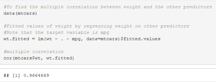
2. R-squared of individual predictors

Consider a problem on linear regression where we have 4 predictors  X1,X2, X3 and X4. Let us use Y to denote the target variable. For each predictor Xi, let us fit a linear regression model to regress Xi on the remaining predictors. This will give us four regression models:

For example, if Ri2 = 0.90, then this would mean that, 90% of variance of X1 is explained by the variables X2, X3 and X4 using model 1. If the value of Ri2 is high, as being discussed in this case, then this would indicate that the ith predictor is redundant because most of its variance is explained by the other predictors. In other words, in the presence of the other predictors the ith predictor does not provide any additional information to explain Y. Therefore, it would be advisable to remove such redundant predictors from the model.

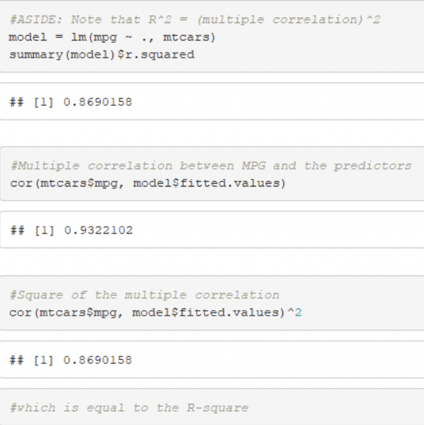
This is a very interesting relationship. This is the reason why R-squared is also known as multiple R-squared. Since, R-squared is the square of multiple correlation, it ranges between 0 and 1. If a predictor is highly collinear with the other predictors then the multiple correlation between the predictor and the rest of the predictors will be closer to +1 or -1 and the value of Ri2 will be closer to 1. 

R Code:

3. VIF (Variance Inflation Factor) 

The VIF or the Variance Inflation Factor for the predictor Xi  is calculated using the following formula:

Note that, though VIF helps in detecting multicollinearity, it is not a measure of multicollinearity. In the next section, we will discuss some details about the formula of VIF and talk about why this formula is called variance inflation factor.

VARIANCE INFLATION FACTOR (VIF)

The coefficients of linear regression are estimated by minimizing the sum of squares of the residuals (RSS). The RSS depends on the collected sample. Therefore, as the sample changes the estimated values of the coefficient changes as well. This dispersion of the linear regression coefficients over different samples is captured by calculating the standard errors of the regression coefficients. The standard errors of the linear regression coefficients are calculated using the following formula.

Rearranging the factors in the above equation will give us,

This is the reason why this factor is called the variance inflation factor (VIF).

Let us do a quick check using a software to see how this formula gives the estimated standard error of a linear regression coefficient.

Quick check using R

In this section, we will calculate the standard error of the estimated coefficient of the of the variable weight using the formula and cross-check with the standard R-output of the linear model.

Note that, the standard error of the estimated coefficient of the of the variable weight in the summary is 1.01547 which matches with the value we obtained using the formula.

VIF calculation using R. These is a simple function in R which can help us to calculate VIFs easily. The function is present in the package cars.

Interpretation of VIF. This is the number by which the variance of the coefficient of the i^th predictor inflates compared to what it would be if R_i = 0, i.e. if the i^th predictor is uncorrelated with the other predictors. For example, VIF corresponding to the variable weight is 15.164. This would mean that the variance of the estimated coefficient of the variable weight inflates by 15.164 times compared to what it would be if the variable weight in uncorrelated with the other predictors.

PROBLEMS DUE TO MULTICOLLINEARITY

In linear regression analysis we perform a t-test to test if a predictor is linearly related to the target. The null and alternate hypothesis of this statistical test are:

compared to a false rejection of the alternate hypothesis (which is the type 2 error). Therefore, before the start of any statistical testing of hypothesis problem we always pre-set the value of  (the probability of the type 1 error) to a very small value. You may be very cautious about committing a type 1 error but believe me you are probably more interested in not making a type 2 error.

Let us understand this with a fictitious example – a medicine company has worked very hard over the past few years to come up with a new drug that claims to cure headache within 5 minutes on the average. In order to support this claim using data a hypothesis framework is needed to be designed and the claim is needed to be tested experimentally.

Now, we need to test these hypotheses experimentally. For example, to keep things simple, let’s say  subjects who suffer from headaches are chosen at random. These patients are kept under some observations and are prescribed to take this new medicine whenever they suffer from headache. The time (in minutes) taken to cure headache for each individual patients are recorded. A very small value of the average of these durations will lead us to suspect our null hypothesis and will give us a very small p value. (Please note that the above mentioned example is a simplified one and experimental designs has lot more to do than just picking a random sample of patients).

A large p value, a value which is at least greater than the level of significance, will lead us to reject H₁. However, the rejection of H₁ does not necessary mean that the claim is false. Based on the sample, that’s the best decision we may take. If H₁ is rejected falsely then we commit a type 2 error. Committing a type 2 error would indicate that the medicine was truly effective but the effect of the medicine could not be captured from the collected sample. However, as an experimental researcher, you would probably like your statistical tests to be designed in such a way that would enable it to capture the effect. The ability of a statistical testing to capture an effect that is present is called the power of a test. In other words, the probability of a statistical test to accept the alternate hypothesis correctly (or, reject the null hypothesis correctly) is called the power of a test. Therefore, mathematically power of a test can be written as,

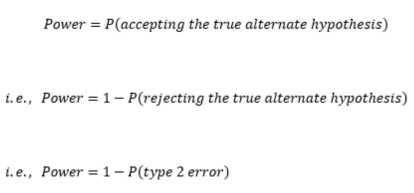
Therefore, the lesser is the probability of type 2 error the more is the power of the statistical test.

Multicollinearity inflates the variance of the linear regression coefficients. Is that a problem?

Now, let’s come back to our discussion on how the presence of multicollinear predictors affects the linear regression analysis.

decreases. This will increase the p value of the test. In this case, we may fail to reject the false null hypothesis correctly and fail to accept the true alternate hypothesis correctly. This increases the probability of committing the type 2 error and hence the power of the statistical test increases.

So, in short, multicollinearity reduced the power of the statistical t-test in linear regression. This may in turn disable us to identify the effect of the individual predictors on the target.