Data Science with a variety of powerful algorithms has a large scope of application in financial analytics. Many financial analytics problems are based on the time-series analysis where a machine learning model is required to predict the values on a time-series pattern. Deep learning models have been applied to a variety of difficult predictive analytics problems. Time series prediction is one of those difficult applications. LSTM Recurrent Neural Networks have proven their capability to outperform in the time series prediction problems. When it comes to learn from the previous patterns and predict the next pattern in the sequence, LSTM models are best in this task.
In this article, we will implement the LSTM Recurrent Neural Network to predict the foreign exchange rate. The LSTM model will be trained to learn the series of previous observations and predict the next observation in the sequence. We will apply this model in predicting the foreign exchange rate of India.
The Data Set
The data set in the experiment is taken from Kaggle that is publicly available as Foreign Exchange Rates 2000-2019. This dataset was originally generated on the Federal Reserve’s Download Data Program. It comprises the exchange rates of 22 countries including the Euro Area for 5217 days.
Implementation
This code was implemented in Google Colab and the .py file was downloaded.
# -*- coding: utf-8 -*-
"""Copy of foreign_exchange.ipynb

Automatically generated by Colaboratory.

Original file is located at
    https://colab.research.google.com/drive/1ItQXXc-Z33hr6W60E6gxxxxxxxxxxxxx
"""
First of all, we will import the Python libraries to be required in this program.
#Importing Libraries
import pandas as pd
import numpy as np
import matplotlib.pyplot as plt
# %matplotlib inline
import tensorflow as tf
import keras
from keras.models import Sequential
from keras.layers import Dense, LSTM
We will read the data set in the program. In Google Colab, the Foreign_Exchange_Rates.csv file was uploaded to the session storage.
#Reading dataset
data_set = pd.read_csv('Foreign_Exchange_Rates.csv', na_values='ND')
Using the next lines of codes, we will see the shape of the data set and the head of the dataset.
#Dataste Shape data_set.shape#Dataset head data_set.head()

We are interested in the foreign exchange rate in India. So, before proceeding further on this data, let us visualize it. Please note that we are not going to change indexing that is required to visualize the dates on the X-axis.
#Plotting Indian Exchange rate
plt.plot(data_set['INDIA - INDIAN RUPEE/US$'])
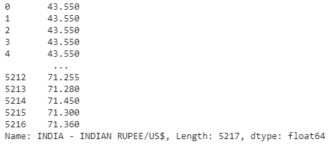
We will specify the data frame of our interest that consists of the foreign exchange rate of India.
#Data frame
df = data_set['INDIA - INDIAN RUPEE/US$']
df
In the next step, we will preprocess the training and test data for the LSTM network. The model will be trained on the sequence of the previous value and the current value.
#Preprocessing data set df = np.array(df).reshape(-1,1) from sklearn.preprocessing import MinMaxScaler scaler = MinMaxScaler() df = scaler.fit_transform(df) print(df)#Training and test sets train = df[:4800] test = df[4800:] print(train.shape) print(test.shape)
def get_data(data, look_back): data_x, data_y = [],[] for i in range(len(data)-look_back-1): data_x.append(data[i:(i+look_back),0]) data_y.append(data[i+look_back,0]) return np.array(data_x) , np.array(data_y) look_back = 1 x_train , y_train = get_data(train, look_back) print(x_train.shape) print(y_train.shape)
x_test , y_test = get_data(test,look_back) print(x_test.shape) print(y_test.shape)
#Processing train and test sets for LSTM model x_train = x_train.reshape(x_train.shape[0],x_train.shape[1], 1) x_test = x_test.reshape(x_test.shape[0],x_test.shape[1], 1) print(x_train.shape) print(x_test.shape)

Using the below lines of codes, we will define the LSTM recurrent neural network and train it on the data prepared above.
#Defining the LSTM model n_features=x_train.shape[1] model=Sequential() model.add(LSTM(100,activation='relu',input_shape=(1,1))) model.add(Dense(n_features)) #Model summary model.summary()#Compiling model.compile(optimizer='adam', loss = 'mse') #Training model.fit(x_train,y_train, epochs = 5, batch_size=1)

Foreign Exchange Rate Prediction
Once the LSTM model is trained, we will apply it to predict the future sequences for the test data.
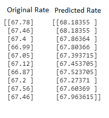
#Prediction using the trained model scaler.scale_ y_pred = model.predict(x_test) y_pred = scaler.inverse_transform(y_pred) print(y_pred[:10])#Processing test shape y_test = np.array(y_test).reshape(-1,1) y_test = scaler.inverse_transform(y_test) print(y_test[:10])
#Visualizing the results plt.figure(figsize=(10,5)) plt.title('Foreign Exchange Rate of India') plt.plot(y_test , label = 'Actual', color = 'g') plt.plot(y_pred , label = 'Predicted', color = 'r') plt.legend()
#Mean Squared Error from sklearn.metrics import mean_squared_error mean_squared_error(y_test, y_pred)

As we can see in the above plot the LSTM model has predicted almost the same sequence as it was expected. The Mean Squared Error obtained is also very less as we can see above. So we can conclude that the model has given accurate predictions about the foreign exchange rate. The same we will see in the below illustration for 10 values.
#10 original and predicted rates together


