Decision trees are one of the most used machine learning models because of their ease of implementation and simple interpretations. To better learn from the data they are applied to, the nodes of the decision trees need to be split based on the attributes of the data. In this article, we will understand the need of splitting a decision tree along with the methods used to split the tree nodes. Gini impurity, information gain and chi-square are the three most used methods for splitting the decision trees. Here we will discuss these three methods and will try to find out their importance in specific cases. The major points that we will cover in this article are outlined below.
Table of Contents
- Decision Tree
- Key Terminologies of Decision Trees
- Node Splitting in Decision Trees
- Decision Tree Splitting Methods
- Gini Impurity
- Information Gain
- Chi-Square
- Comparing the Splitting Methods
Let’s start the discussions with understanding the decision trees.
Decision Tree
One of the predictive modelling methodologies used in machine learning is decision tree learning, also known as induction of decision trees. It goes from observations about an item (represented in the branches) to inferences about the item’s goal value (represented in the leaves) using a decision tree (as a predictive model).
Classification trees are tree models in which the goal variable can take a discrete set of values; in these tree structures, leaves indicate class labels and branches represent feature combinations that lead to those class labels. Regression trees are decision trees in which the target variable has a range of values (usually real numbers). Given their comprehensibility and simplicity, decision trees are one of the most popular machine learning methods.
The primary idea behind a decision tree is to find the features that hold the most information about the target feature and then partition the dataset along with the values of these features, resulting in target feature values that are as pure as possible at the nodes. The most informative feature is one that best isolates the uncertainty from information about the target feature. The search process for a most informative characteristic goes on until we end up with pure leaf nodes.
Key Terminologies of Decision Trees
Let’s have a look at what a decision tree looks like and how it works when a fresh input for prediction is provided. The graphic below depicts the basic construction of the decision tree. Every tree has a root node via which the inputs are routed. This root node is subdivided further into sets of decision nodes where findings and observations are conditionally based.
Splitting is the process of dividing a single node into numerous nodes. If a node does not split into other nodes, it is referred to as a leaf node or terminal node. A branch or sub-tree is a segment of a decision tree. There is another concept that is diametrically opposed to splitting.
Cases are classified by decision trees by sorting them along the tree from the root to some leaf/terminal node, with the leaf/terminal node categorizing the example. Each node in the tree is a test case for some property, and each edge descending from the node represents one of the possible solutions to the test case. This is a recursive process that is repeated for each new node-rooted subtree.
Node Splitting in Decision Trees
Decision trees are totally dependent on the objective variable, although their algorithms differ from those used for classification and regression trees. There are numerous approaches for deciding how to partition the provided data.
The primary purpose of decision trees is to find the best splits between nodes that will best divide the data into the appropriate categories. To accomplish this, we must employ the proper decision-making procedures. The rules have a direct impact on the algorithm’s performance.
There are a few assumptions that must be made:
- The entire data set is considered the root at first, and then we utilize methods to break or divide the root into subtrees.
- The feature values are classified as categorical. If the values are continuous, they are split before the model is built.
- Recursively, records are distributed based on attribute values.
- A statistical approach is used to order characteristics as the tree’s root or an internal node.
Decision Tree Splitting Methods
It’s tough to decide which variables to put at the root or at different levels of the tree as internal nodes when the dataset comprises N variables. Choosing any node as the root at random will not solve the problem. We can receive disappointing results with limited precision if we use a random technique. Researchers collaborated to develop answers to the attribute selection challenge. They recommended employing criteria such;
- Gini Impurity
- Information Gain
- Chi-Square
Each attribute’s value will be calculated using these criteria. The values are sorted, and characteristics are ordered in the tree, with the attribute having the highest value (in the case of information gain) at the top. We assume categorical attributes for Information Gain and continuous attributes for the Gini impurity.
Gini Impurity
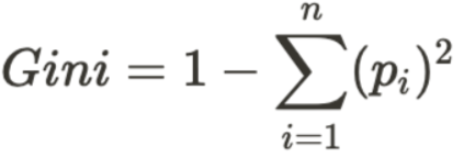
The division is called pure if all elements are accurately separated into different classes (an ideal scenario). The Gini impurity (pronounced “genie”) is used to predict the likelihood that a randomly selected example would be incorrectly classified by a specific node. It is called an “impurity” metric because it shows how the model differs from a pure division.
The degree of Gini impurity ranges from 0 to 1, with 0 indicating that all of the elements belong to a single class and 1 indicates that only one class exists. The Gini impurity of value 1 indicates that all of the items are randomly distributed over various classes, whereas a value of 0.5 indicates that the elements are uniformly distributed across some classes. It is stated as given below formula originally by Leo Breiman in 1984.
How to Calculate the Gini Impurity for a Split
- Calculate Gini for sub-nodes using the aforementioned success(p) and failure(q) formulas (p2+q2).
- Calculate the Gini Impurity for each split node using the weighted Gini score.
Information Gain
The concept of entropy is crucial in gauging information gain. “Information gain, on the other hand, is based on information theory.” The term “information gain” refers to the process of selecting the best features/attributes that provide the most information about a class. It adheres to the concept of entropy while attempting to reduce the level of entropy from the root node to the leaf nodes. The difference in entropy before and after splitting is computed as information gain, which specifies the impurity of in-class elements.
Information Gain = 1 – Entropy
Entropy is a measure of a random variable’s uncertainty; it characterizes the impurity of any arbitrary collection of samples. The higher the entropy, the more information there is.
When we employ a node in a decision tree to segment the training instances into smaller subsets, the entropy often changes. The change in entropy is measured by information gain.
Sklearn supports the “entropy” requirement for Information Gain, and we must explicitly express it if we wish to use the Information Gain method in sklearn.
The following are the steps to divide a decision tree using Information Gain:
- Calculate the entropy of each child node separately for each split.
- As the weighted average entropy of child nodes, compute the entropy of each split.
- Choose the split that has the lowest entropy or the biggest information gain.
- Repeat steps 1-3 until you have homogeneous nodes.
Chi-Square
CHAID is an abbreviation for Chi-squared Automatic Interaction Detector. It is one of the oldest systems of tree classification. It determines the statistical significance of differences between sub-nodes and the parent node. The sum of squares of the standardized discrepancies between the observed and expected frequencies of the target variable is used to calculate it.

It operates on the categorical target variable “Success” or “Failure.” It is capable of performing two or more splits. The greater the Chi-Square value, the greater the statistical significance of discrepancies between sub-node and Parent nodes.
Another major benefit of utilizing chi-square is that it can do numerous splits at a single node, resulting in greater precision and accuracy. To calculate the Chi-square for a split, follow these steps:
- Take the sum of the Chi-Square values for each class in a node to determine the Chi-Square value of each child node for each split.
- Calculate each split’s Chi-Square value as the total of all the child node’s Chi-Square values.
- Choose the split that has the greater Chi-Square value.
- Steps 1-3 should be repeated until you have homogeneous nodes.
Comparing the Splitting Methods
In the following, we will go through some comparison points drawn from the above discussion which will help to decide which method is to use.
- Information gain is calculated by multiplying the probability of a class by the log base 2 of that class probability. Gini impurity is calculated by subtracting the sum of the squared probabilities of each class from one.
- The Gini Impurity favours bigger partitions (distributions) and is simple to implement, whereas information gains favour smaller partitions (distributions) with a variety of diverse values, necessitating a data and splitting criterion experiment.
- When working with categorical data variables, the Gini Impurity returns either “success” or “failure” and solely does binary splitting; in contrast, information gain evaluates the entropy differences before and after splitting and illustrates impurity in class variables.
- Chi-square aids in determining the statistical significance of differences between sub-nodes and the parent node. We calculate it as the sum of the squares of the standardized discrepancies between the observed and expected frequencies of the target variable.
Final Words
Through this post, we have seen what are different methods can be used in the background working of a decision tree algorithm. We also discussed how decision trees split and what are the different approaches used for decision tree splits. We also went through many important terminologies related to trees and discussed all those methods in detail.


