In our previous article, we detailed out the need for Trusted AI and discussed one of IBM Research Trusted AI toolkit called AIF360. I recommend you to read this article first for better understanding. In this article, we are going to discuss about AI Explainability 360 toolkit.

The growing interactions of the world with AI systems has pushed AI into all kinds of rigid domains(Agriculture, Law, Administration, etc) making predictions for society in all aspects(loan approval, cancer detection, etc). This has increased the onus of AI systems for being more reliable and accurate and providing a precise explanation for their decision-making process.  These explanations allow users to get an insight into how a machine thinks which is important to gain trust and confidence in AI systems. This has set off a growing community of researchers, developing interpretable or explainable AI systems.

Though many algorithms and tools have come out, there is still a gap between what users want and what researchers are producing. The reason for this is the vague definition of an explanation. For instance, if a doctor tries to understand an AI system for cancer detection, he/she will look for a similar case and then conclude their result; If a person got rejected for loan application, he/she want to know the reasons behind it; However, if developers/ scientists deals with these case, they would want to understand where these AI models more or less confident as a means of improving its performance. Hence, we require some organizing principles and tools that can take account for different explanations, to solve this problem.

Keeping the above dilemma in mind, the research of IBM has come up with an AI Explainability 360(AIX 360 – One Explanation Does Not Fit All) toolkit. It is an open-source toolkit which takes account many possible explanations for consumers. The goal is to demonstrate how different explainability methods can be applied in real-world scenarios. It provides interpretability and explainability of datasets and machine learning models. The package for this toolkit is available in Python and includes a comprehensive set of algorithms that cover different dimensions of explanations along with explainability metrics. It gives the taxonomy of selecting the best possible explanation for the data as well as for models. Please refer to this link for the terminologies required in this session. There is no single approach to explainability. There are many ways to explain how machine learning makes predictions such as:

• data vs. model
• directly interpretable vs. post hoc explanation
• local vs. global
• static vs. interactive

Given below is the required taxonomy for selecting the explanation algorithm, provided by AI Explainability 360.

There are eight state-of-the-art explainability algorithms that are added in AI Explainability 360 toolkit.

• ProtoDash (Gurumoorthy et al., 2019)
• Contrastive Explanations Method (Dhurandhar et al., 2018)
• Contrastive Explanations Method with Monotonic Attribute Functions (Luss et al., 2019)
• LIME (Ribeiro et al. 2016, Github)
• SHAP (Lundberg, et al. 2017, Github)
• Teaching AI to Explain its Decisions (Hind et al., 2019)
• Boolean Decision Rules via Column Generation (Light Edition) (Dash et al., 2018)
• Generalized Linear Rule Models (Wei et al., 2019)
• ProfWeight (Dhurandhar et al., 2018)

Supported explainability metrics are:

• Faithfulness (Alvarez-Melis and Jaakkola, 2018)
• Monotonicity (Luss et al., 2019)

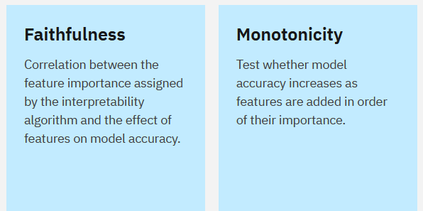
Let’s jump into the implementation part.

Requirements

1. Python>=3.6
2. Install the AIX 360 library through pip

!pip install aix360

Introduction to Dataset

For demo purposes, we are going to take a Credit Approval problem explaining different types of explanations required for data scientists, loan officers and bank customers. The dataset which we are going to use is the FICO Explainable Machine Learning Challenge. The dataset can be downloaded by filling the google form here (for licensing) and an email will be sent to your registered email id containing the dataset and data dictionary. The details of the dataset can be found here. The machine learning task for this dataset is to predict whether a customer has made payment within the time period or not. The target variable is RiskPerformance. The value “bad” indicates that the customer took more than 90 days for their due payments within 24 months of the account being open and the value “good” implies its opposite. The relationship between predictor variables and target variable is indicated by Monotonicity Constraint with the probability of bad equals to 1. If the value of this constraint is monotonically decreasing then as the value of variable increases, the probability of loan application being “bad” decreases.

Credit Loan Approval – Explanation for Data Scientists

1. Load the Heloc Dataset through AI Explainability 360 with custom_preprocessing equal to nan_preprocessing(convert special values to np.nan) which can directly be handled by AIX 360 algorithms(without replacing). Then split the data into train set and test set via sklearn.

# Load FICO HELOC data with special values converted to np.nan
from aix360.datasets.heloc_dataset import HELOCDataset, nan_preprocessing
data = HELOCDataset(custom_preprocessing=nan_preprocessing).data()
# Separate target variable
y = data.pop('RiskPerformance')
# Split data into training and test sets using fixed random seed
from sklearn.model_selection import train_test_split
dfTrain, dfTest, yTrain, yTest = train_test_split(data, y, random_state=0, stratify=y)
dfTrain.head().transpose()

2. We are going to use Boolean Decision Rules via Column Generation(BRCG) and LogRR algorithms which require binary features. Hence, converting non-binarized features to binary form with the help of FeatureBinarizer class. The values are divided into 10 bins including all the continuous and negation values.

# Binarize data and also return standardized ordinal features
from aix360.algorithms.rbm import FeatureBinarizer
fb = FeatureBinarizer(negations=True, returnOrd=True)
##return standardized versions of the original unbinarized ordinal features, which are used by LogRR but not BRCG
dfTrain, dfTrainStd = fb.fit_transform(dfTrain)
dfTest, dfTestStd = fb.transform(dfTest)
#Below is the result of binarizing the first 'ExternalRiskEstimate' feature.
dfTrain['ExternalRiskEstimate'].head()

3. BRCG is used to produce simple OR-of-Ands rule(disjunctive normal form, DNF) for binary classification. Here a DNF represents a whole rule set, where AND clause shows the individual value. Column Generation is used to generate promising results by searching for all possible rule sets.  For this dataset, we have used CNF(conjunctive normal rule)

# Instantiate BRCG with small complexity penalty and large beam search width
from aix360.algorithms.rbm import BooleanRuleCG
# The model complexity parameters lambda0 and lambda1 penalize the number of clauses in the
#rule and the number of conditions in each clause. 
# We use the default values of 1e-3 for lambda0 and lambda1 
#(decreasing them did not increase accuracy here) and leave other parameters at their defaults as well. 
# The model is then trained, evaluated, and printed.
br = BooleanRuleCG(lambda0=1e-3, lambda1=1e-3, CNF=True)

# Train, print, and evaluate model
br.fit(dfTrain, yTrain)
from sklearn.metrics import accuracy_score
print('Training accuracy:', accuracy_score(yTrain, br.predict(dfTrain)))
print('Test accuracy:', accuracy_score(yTest, br.predict(dfTest)))
print('Predict Y=0 if ANY of the following rules are satisfied, otherwise Y=1:')
print(br.explain()['rules'])

Here, ExternalRiskEstimate represents a consolidated version of risk markers(higher is better)and NumSatisfactoryTrades represents a number of satisfactory credit accounts. If the value of y is a “1” then the person defaulted on the loan. If the value is a “0” then the person paid back the loan. Point to be noted that with these two clauses including the same features, we are able to generate a pretty decent accuracy of 69.65%.

4. Next we fit and evaluate the LogRR model, which improves the accuracy by making the model a bit complex. It fits a logistic regression algorithm using rule-based features. 

# Instantiate LRR with good complexity penalties and numerical features
from aix360.algorithms.rbm import LogisticRuleRegression
# Here we are also including unbinarized ordinal features (useOrd=True) in addition to rules. 
# Similar to BRCG, the complexity parameters lambda0, lambda1 penalize the number of rules included in the model and the number of conditions in each rule. 
# The values for lambda0, lambda1 below strike a good balance between accuracy and model complexity.

lrr = LogisticRuleRegression(lambda0=0.005, lambda1=0.001, useOrd=True)

# Train, print, and evaluate model
lrr.fit(dfTrain, yTrain, dfTrainStd)
print('Training accuracy:', accuracy_score(yTrain, lrr.predict(dfTrain, dfTrainStd)))
print('Test accuracy:', accuracy_score(yTest, lrr.predict(dfTest, dfTestStd)))
print('Probability of Y=1 is predicted as logistic(z) = 1 / (1 + exp(-z))')
print('where z is a linear combination of the following rules/numerical features:')
lrr.explain()

The test accuracy of the LogRR model is slightly better than the BRCG. The model created all the rules with single conditions only, no interactions are made between the features. Hence, it is a kind of generalized additive model (GAM). Next, we will see the plotting of univariate functions that make it as GAM.

5. With the help of the visualize() method of LogRR model, we will plot all the first degree rules. Out of 36 features, 14(excluding intercept) features are single conditioned. Check here all the plots and its explanation. An example of it is shown below

You can check the full demo for this, here.

Credit Loan Approval – Explanation for Loan Officers

In this section, we will take an algorithmic approach to give explanations for the AI model that will help Loan officers understand the black box ML. For this, we will try to find similar user profiles for an applicant obtained by Protodash Algorithm. This algorithm selects the application from the training dataset that is similar to the applicant, we want to explain and this similarity is found in different ways(by matching the distribution), unlike nearest neighbour techniques. Hence, Protodash gives a wholesome view to answer why the particular decision has been made.

We will see two cases: One, where the application has been approved. Second, where the application has been rejected. In each case, the top five prototypes from the training data along with the similarity factor will be explained.

1. Import the required libraries and framework

#Import necessary libraries, frameworks and algorithms.
import pandas as pd
import numpy as np
import tensorflow as tf
from keras.models import Sequential, Model, load_model, model_from_json
from keras.layers import Dense
import matplotlib.pyplot as plt
from IPython.core.display import display, HTML
 
from aix360.algorithms.contrastive import CEMExplainer, KerasClassifier
from aix360.algorithms.protodash import ProtodashExplainer
from aix360.datasets.heloc_dataset import HELOCDataset

2. Load the dataset and show some sample applicants.

# Clean data and split dataset into train/test
(Data, x_train, x_test, y_train_b, y_test_b) = heloc.split()
 
#Normalize the dataset
Z = np.vstack((x_train, x_test))
Zmax = np.max(Z, axis=0)
Zmin = np.min(Z, axis=0)
 
#normalize an array of samples to range [-0.5, 0.5]
def normalize(V):
    VN = (V - Zmin)/(Zmax - Zmin)
    VN = VN - 0.5
    return(VN)
    
# rescale a sample to recover original values for normalized values. 
def rescale(X):
    return(np.multiply ( X + 0.5, (Zmax - Zmin) ) + Zmin)
 
N = normalize(Z)
xn_train = N[0:x_train.shape[0], :]
xn_test  = N[x_train.shape[0]:, :]

4. Define the Neural Network and train the dataset. The architecture of neural network can be defined as:

#this is the architecture of a 2-layer neural network classifier whose predictions we will try to interpret.
# nn with no softmax
def nn_small():
    model = Sequential()
    model.add(Dense(10, input_dim=23, kernel_initializer='normal', activation='relu'))
    model.add(Dense(2, kernel_initializer='normal'))    
    return model   

Now. train this neural network.

# Set random seeds for repeatability
np.random.seed(1) 
tf.set_random_seed(2) 
 
class_names = ['Bad', 'Good']
 
# loss function
def fn(correct, predicted):
    return tf.nn.softmax_cross_entropy_with_logits(labels=correct, logits=predicted)
 
# compile and print model summary
nn = nn_small()
nn.compile(loss=fn, optimizer='adam', metrics=['accuracy'])
nn.summary()
 
# train model or load a trained model
TRAIN_MODEL = True
 
if (TRAIN_MODEL): 
    nn.fit(xn_train, y_train_b, batch_size=128, epochs=500, verbose=1, shuffle=False)
    nn.save_weights("heloc_nnsmall.h5")     
else:    
    nn.load_weights("heloc_nnsmall.h5")
        
# evaluate model accuracy        
score = nn.evaluate(xn_train, y_train_b, verbose=0) #Compute training set accuracy
#print('Train loss:', score[0])
print('Train accuracy:', score[1])
 
score = nn.evaluate(xn_test, y_test_b, verbose=0) #Compute test set accuracy
#print('Test loss:', score[0])
print('Test accuracy:', score[1])

5. Obtaining similar applicants whose application got approved.

#normalize the data and chose a particular applicant, whose profile is displayed below
p_train = nn.predict_classes(xn_train) # Use trained neural network to predict train points
p_train = p_train.reshape((p_train.shape[0],1))
 
z_train = np.hstack((xn_train, p_train)) # Store (normalized) instances that were predicted as Good
z_train_good = z_train[z_train[:,-1]==1, :]
 
zun_train = np.hstack((x_train, p_train)) # Store (unnormalized) instances that were predicted as Good 
zun_train_good = zun_train[zun_train[:,-1]==1, :]

Now, we will choose applicant 8 whose application got approved. The explanation for these will be provided by Protodash Algorithm.

##Let us now consider applicant 8 whose loan was approved. 
#Note that this applicant was also considered for the contrastive explainer, however, 
#we now justify the approved status in a different manner using prototypical examples, 
#which is arguably a better explanation for a bank employee.
 
idx = 8
 
X = xn_test[idx].reshape((1,) + xn_test[idx].shape)
 
print("Chosen Sample:", idx)
print("Prediction made by the model:", class_names[np.argmax(nn.predict_proba(X))])
print("Prediction probabilities:", nn.predict_proba(X))
print("")
 
# attach the prediction made by the model to X
X = np.hstack((X, nn.predict_classes(X).reshape((1,1))))
 
Xun = x_test[idx].reshape((1,) + x_test[idx].shape) 
dfx = pd.DataFrame.from_records(Xun.astype('double')) # Create dataframe with original feature values
dfx[23] = class_names[int(X[0, -1])]
dfx.columns = df.columns
dfx.transpose()

Now, fitting the protodash algorithm to find the similar applicants predicted as “Good”.

#Find similar applicants predicted as "good" using the protodash explainer.
explainer = ProtodashExplainer()
(W, S, setValues) = explainer.explain(X, z_train_good, m=5) # Return weights W, Prototypes S and objective function values

Display similar applicants along with similarity factors labelled as “weights”.

## Display similar applicant user-profiles and the extent to which they are similar to the chosen applicant
##as indicated by the last row in the table below labelled as "Weight"
 
dfs = pd.DataFrame.from_records(zun_train_good[S, 0:-1].astype('double'))
RP=[]
for i in range(S.shape[0]):
    RP.append(class_names[int(z_train_good[S[i], -1])]) # Append class names
dfs[23] = RP
dfs.columns = df.columns  
dfs["Weight"] = np.around(W, 5)/np.sum(np.around(W, 5)) # Calculate normalized importance weights
dfs.transpose()

Now, compute and display the similarity of features of prototypical users to the chosen applicant. The closer the value to 1, the more similar the features of prototypical users to the chosen applicant.

# ##Compute how similar a feature of a prototypical user is to the chosen applicant.
# The more similar the feature of prototypical user is to the applicant, the closer its weight is to 1.
# We can see below that several features for prototypes are quite similar to the chosen applicant. 
# A human friendly explanation is provided thereafter.
z = z_train_good[S, 0:-1] # Store chosen prototypes
eps = 1e-10 # Small constant defined to eliminate divide-by-zero errors
fwt = np.zeros(z.shape)
for i in range (z.shape[0]):
    for j in range(z.shape[1]):
        fwt[i, j] = np.exp(-1 * abs(X[0, j] - z[i,j])/(np.std(z[:, j])+eps)) # Compute feature similarity in [0,1]
                
# move wts to a dataframe to display
dfw = pd.DataFrame.from_records(np.around(fwt.astype('double'), 2))
dfw.columns = df.columns[:-1]
dfw.transpose() 

    The output of above code is displayed below:

The above table displays the five closed user profiles for the chosen applicant. We can conclude from the table that, out of 5 user profiles, the user 0 is the most similar applicant to the given user(12 out of 23 features are exactly similar i.e., weight is equal to 1). In all, this table strongly proves that the chosen applicant is no defaulter. Hence, giving more trust to Loan Officers to mark the application as “approved”.

6. Similarly, we can give explanations for a rejected applicant. The code for this is similar to the approved applicant, you can check the code snippet here.

You can check the full demo, here.

Credit Loan Approval – Explanation for Customers

In this part of the demo, we are going to compute explanations for end-users(customers) of AI systems that can make users understand why their application is approved or rejected and what are the required changes to change the decision of AI model from reject to approve. Apart from that, organizations(banks, financial institutes, etc.) also want to understand the approach of the AI model in approving or rejecting the application. We will try to find out these contrastive explanations with help of Explanations based on the Missing: Towards Contrastive Explanations with Pertinent Negatives algorithm. This algorithm consists of two parts:

a) Pertinent Negatives (PNs): It identifies a minimal set of features which if altered would change the classification of the original input. For example, in this case if a person’s credit score is increased their loan application status may change from reject to accept.

 b) Pertinent Positives (PPs) : It  identifies a minimal set of features and their values that are sufficient to yield the original input’s classification. For example, an individual’s loan may still be accepted if the salary was 50K as opposed to 100K.

For more details of this algorithm, please refer to the above link. The initial 4 steps for generating contrastive explanations are the same as we discussed in this section.

1. Import the required libraries and framework(same as above).
2. Load the dataset and show some sample applicants( same as above).
3. Preprocess and normalize the Heloc dataset for training(same as above).
4. Define the Neural Network and train the dataset(same as above).
5. Now, compute the contrastive explanation for a few applicants. For the first part, we will select the applicants whose application was rejected and will try to find out the minimal change required to change the status to approved(by calculating Pertinent Negatives). For the second part. We will select the applicants whose application was approved and will try to find the minimal values of features that will yield the same result(i.e., calculating Positive Pertinent).

First, the computer PN’s CEM explainer will calculate the similar user profiles(for chosen applicants) whose result is not the same as the chosen applicant. This explainer will change the minimal set of features to a minimal amount and try to learn on what changes, the chosen application got selected.

# In order to compute pertinent negatives, the CEM explainer computes a user profile that is close to the original applicant but 
# for whom the decision of HELOC application is different. The explainer alters a minimal set of features by a minimal (positive) amount. 
# This will help the user whose loan application was initially rejected say, to ascertain how to get it accepted.
 
# Some interesting user samples to try: 2344 449 1168 1272
idx = 1272
 
X = xn_test[idx].reshape((1,) + xn_test[idx].shape)
print("Computing PN for Sample:", idx)
print("Prediction made by the model:", nn.predict_proba(X))
print("Prediction probabilities:", class_names[np.argmax(nn.predict_proba(X))])
print("")
 
mymodel = KerasClassifier(nn)
explainer = CEMExplainer(mymodel)
 
arg_mode = 'PN' # Find pertinent negatives
arg_max_iter = 1000 # Maximum number of iterations to search for the optimal PN for given parameter settings
arg_init_const = 10.0 # Initial coefficient value for main loss term that encourages class change
arg_b = 9 # No. of updates to the coefficient of the main loss term
arg_kappa = 0.2 # Minimum confidence gap between the PNs (changed) class probability and original class' probability
arg_beta = 1e-1 # Controls sparsity of the solution (L1 loss)
arg_gamma = 100 # Controls how much to adhere to a (optionally trained) auto-encoder
my_AE_model = None # Pointer to an auto-encoder
arg_alpha = 0.01 # Penalizes L2 norm of the solution
arg_threshold = 1. # Automatically turn off features <= arg_threshold if arg_threshold < 1
arg_offset = 0.5 # the model assumes classifier trained on data normalized
                # in [-arg_offset, arg_offset] range, where arg_offset is 0 or 0.5
# Find PN for applicant 1272
(adv_pn, delta_pn, info_pn) = explainer.explain_instance(X, arg_mode, my_AE_model, arg_kappa, arg_b,
                                                         arg_max_iter, arg_init_const, arg_beta, arg_gamma,
                                                            arg_alpha, arg_threshold, arg_offset)

Now, we will examine an applicant whose application got rejected, with the help of PN’s. We will also generate the importance of each feature to convert the result from negative to positive.

 # Let us start by examining one particular loan application that was denied for applicant 1272. 
# We showcase below how the decision could have been different through minimal changes to the profile conveyed by the pertinent negative.
#  We also indicate the importance of different features to produce the change in the application status. 
# The column delta in the table below indicates the necessary deviations for each of the features to produce this change. 
# A human friendly explanation is then provided based on these deviations following the feature importance plot.
 
#copying the negative peritnent value to a new variable
Xpn = adv_pn
classes = [ class_names[np.argmax(nn.predict_proba(X))], class_names[np.argmax(nn.predict_proba(Xpn))], 'NIL' ]
 
print("Sample:", idx)
#Making prediction based on the original features
print("prediction(X)", nn.predict_proba(X), class_names[np.argmax(nn.predict_proba(X))])
#Making predictions based on the altered features
print("prediction(Xpn)", nn.predict_proba(Xpn), class_names[np.argmax(nn.predict_proba(Xpn))] )
 
 
X_re = rescale(X) # Convert values back to original scale from normalized
Xpn_re = rescale(Xpn)
Xpn_re = np.around(Xpn_re.astype(np.double), 2)
 
delta_re = Xpn_re - X_re
delta_re = np.around(delta_re.astype(np.double), 2)
delta_re[np.absolute(delta_re) < 1e-4] = 0
 
X3 = np.vstack((X_re, Xpn_re, delta_re))
 
dfre = pd.DataFrame.from_records(X3) # Create dataframe to display original point, PN and difference (delta)
dfre[23] = classes
 
dfre.columns = df.columns
dfre.rename(index={0:'X',1:'X_PN', 2:'(X_PN - X)'}, inplace=True)
dfret = dfre.transpose()
 
 
def highlight_ce(s, col, ncols):
    if (type(s[col]) != str):
        if (s[col] > 0):
            return(['background-color: yellow']*ncols)    
    return(['background-color: white']*ncols)
 
dfret.style.apply(highlight_ce, col='(X_PN - X)', ncols=3, axis=1) 

The output of the above code is the table indicating all the altered values in feature to generate the required change in result. The last column (X_PN-X) details out the necessary deviation required for the required change. The value “0” indicates that no change is required.

Now, to translate these changes(from above table) in an easier way(for the customer), we will plot the above table and try to find out the importance of each PN feature. The code snippet is available here.

This indicates that the applicant 1272’s loan application would have been accepted if:

• ExternalRiskEstimate(credit score risk) increased from 65 to 81.
• AverageMInFile increased from 52 months to 66 months.
• And lastly, NumSatisfactoryTrades increased from 17 to 21.

The above changes reflect that the chance of application being approved may increase. It does not guarantee the required change in result.

6. Similarly, we can calculate the Positive pertinents to know about the minimal sufficient values of each feature, keeping the result the same in this case. It will be opposite to what we did for Negative Pertinents. The code snippet for this is available here and the table generated is shown below.

In the above table, the yellow marks in X_PP represent the minimal values of each feature that won’t affect the result. Here, value “0” represents that those features are not important. The whole table can be summarised in the graph below.

This graph indicates that the 9’s loan application would remain accepted if there is:

• No change in ExternalRiskEstimate, AverageMInFile, NumSatisfactoryTrades, PercentTradesNeverDelq
• And the value of MaxDelqEver is at least 2.

You can check the full demo of this, here.

Endnotes

• Colab Notebook AI Explainability 360 – For data scientist explanation
• Colab Notebook AI Explainability 360 – For Loan officer explanation
• Colab Notebook AI Explainability 360 – For Customer explanation

Other examples of using AIX 360 are:

• Medical Expenditure
• Dermoscopy
• Health and Nutrition Survey
• Proactive Retention

You can check other toolkits developed by IBM Research Trusted AI here:

• AI Fairness 360(article)
• Adversarial Robustness 360(article)
• AI FactSheets(article)

Resources and tutorial used above:

• Research Paper
• Github
• Website
• Official Tutorials
• Video Tutorial