Data and proper Analysis of Data can help discover a lot of previously undiscovered factors. The importance of data analytics in any sector that deals with data are highly impactful and essential. It helps create enormous quantities of knowledge that can provide useful insights into each field. In the last ten years, such benefits have led to a surge and a rift in the data market. In order to gain accurate decision making insights, the compilation of data can be made the best use of by its analysis. Data analytics help organizations and businesses to gain insight into a deep sea of knowledge they’d need for further production and growth. Data analytics can be generally applied to all processes and resources necessary for collecting and analysing big critical data.
Analytics is a wider concept, which comprises and incorporates multiple data processing methods and their necessary processes. Analytical methods may be both qualitative and objective. One of the most talked-about analytical methods has been in the domain of Principal Component Analysis. Principal component analysis, known as Karhunen-Loeve or Hotelling transform, belongs to a class of linear transforms based on statistical techniques. This method provides a powerful tool for data analysis and pattern recognition, which is often preferred in signal and image processing as a technique for data compression, data dimension reduction, or decorrelation.
Various algorithms are essentially based on multivariate analysis or neural networks that can perform PCA on a given dataset. Principal component analysis, or PCA, simplifies the major complexity in high dimensional data while retaining trends and patterns. It does so by transforming and reducing the data into fewer dimensions, later acting as summaries of features. High dimensional data is very common these days and consists of multiple features. A principal component can be further defined as a linear combination of optimally weighted observed variables. The output of PCA is principal components, which are less than or equal to the number of original variables. Less, in a case when we wish to discard or reduce the dimensions in our dataset.
PCA is an unsupervised learning method similar to clustering. It finds patterns without prior knowledge about whether the samples come from different treatment groups or essential differences. The objective is pursued by analysing principal components where we can perceive relationships that would otherwise remain hidden in higher dimensions. The representation processed must be such that the loss of information must be minimal after discarding the higher dimensions. The analysis of principal components can reveal relationships between variables and facilitate the dispersion of observations, highlighting possible groupings and detecting the variables that might be responsible for the dispersion. The goal of the methods is to reorient the data so that a multitude of original variables can be summarized with relatively few “factors” or “components” that capture the maximum possible information from the original variables.
Using PCA For Image Reconstruction
Generally, images consist of a lot of pixels that help retain their clarity. Still, as the number of images to process increases its size, it can significantly slow down the system’s performance. We can use the Image Reconstruction technique to overcome this situation, which comes under Unsupervised Machine Learning. Data volume reduction is a common task in image processing. There are a large number of algorithms based on various principles leading to image compression and reconstruction. Also, certain algorithms based on the image colour reduction are lossy, but the results can still be acceptable for some applications. The image transformation technique from colour to the grey level, i.e. the intensity of the image, can be done using most of the common algorithms. According to relation, the implementation is usually based on the weighted sum of three core colour components Red, Green, and Blue. The R, G and B matrices contain image colour components, and the weights are determined regarding the possibilities of human perception.
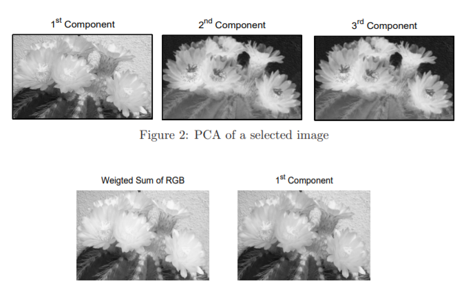
The PCA method provides an alternative way to this method, where the matrix A is replaced by matrix Al where only l largest (instead of n) eigenvalues are used for its formation. A vector of reconstructed variables is then given by relation. A selected real picture P and Its three reconstructed components are obtained accordingly for each eigenvalue and presented. The comparison of the intensity of images obtained from the original image as the weighted colour sum is evaluated as the first principal component. The variance figures for each principal component are present in the eigenvalue list. These indicate the amount of variation accounted for by each component within the feature space.

Getting Started with the Code
In this article, we will perform different image reconstruction methods the Principal Component Analysis Technique can offer and see how an image can be reconstructed to capture maximum information and variance from the image data. Using these techniques, we’ll assess how much visual information we retained as we reconstruct the image from the limited number of Principal Components.
Importing the Libraries
First, let’s import our required libraries that will be essential to test our reconstruction; the following lines of code can be run to do so,
#importing Libraries
import numpy as np
from matplotlib.image import imread
import matplotlib.pyplot as plt
Here we will be using imread from matplotlib to import the image as a matrix.
#setting image path
my_image = imread("/content/5d10e5939c5101174c54bb98.png")
print(my_image.shape)

# Displaying the image
plt.figure(figsize=[12,8])
plt.imshow(my_image)
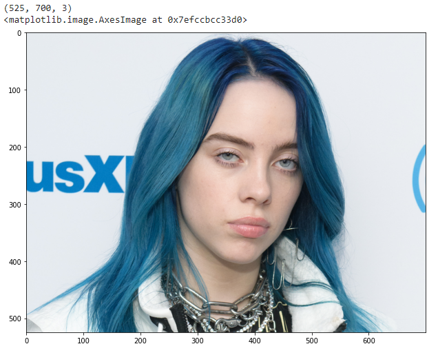
The image being processed is a coloured image and hence has data in 3 channels- Red, Green, Blue. Therefore the shape of the data – 525 x 700 x 3.
Processing the Image
Let us now start with our image processing. Here first, we will be grayscaling our image, and then We’ll perform PCA on the matrix with all the components. We will also create and look at the scree plot to assess how many components we could retain and how much cumulative variance they capture.
#greyscaling the image
image_sum = my_image.sum(axis=2)
print(image_sum.shape)

new_image = image_sum/image_sum.max()
print(new_image.max())

plt.figure(figsize=[12,8])
plt.imshow(new_image, cmap=plt.cm.gray)

#creating scree plot
from sklearn.decomposition import PCA, IncrementalPCA
pca = PCA()
pca.fit(new_image)

# Getting the cumulative variance

var_cumu = np.cumsum(pca.explained_variance_ratio_)*100

# How many PCs explain 95% of the variance?
k = np.argmax(var_cumu>95)
print("Number of components explaining 95% variance: "+ str(k))
#print("\n")

plt.figure(figsize=[10,5])
plt.title('Cumulative Explained Variance explained by the components')
plt.ylabel('Cumulative Explained variance')
plt.xlabel('Principal components')
plt.axvline(x=k, color="k", linestyle="--")
plt.axhline(y=95, color="r", linestyle="--")
ax = plt.plot(var_cumu)
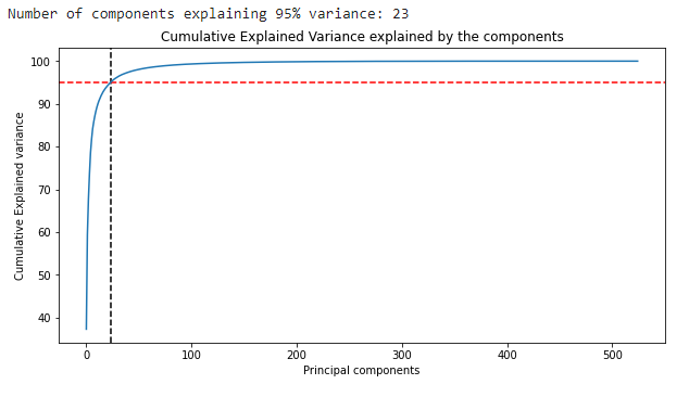
Now let’s reconstruct the image using only 23 components and see if our reconstructed image comes out to be visually different from the original image.
#Reconstructing using Inverse Transform
ipca = IncrementalPCA(n_components=k)
image_recon = ipca.inverse_transform(ipca.fit_transform(new_image))

# Plotting the reconstructed image
plt.figure(figsize=[12,8])
plt.imshow(image_recon,cmap = plt.cm.gray)
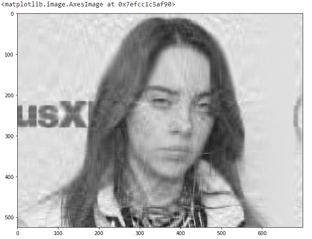
As we can observe, there is a relative difference now. We shall try with a different value of components to check if that makes a difference in the missing clarity and help capture finer details in the visuals.
# Function to reconstruct and plot image for a given number of components

def plot_at_k(k):
    ipca = IncrementalPCA(n_components=k)
    image_recon = ipca.inverse_transform(ipca.fit_transform(new_image))
    plt.imshow(image_recon,cmap = plt.cm.gray)


k = 150
plt.figure(figsize=[12,8])
plot_at_k(100)
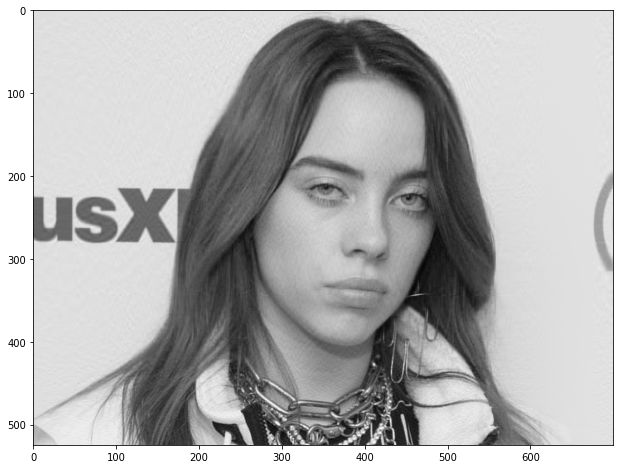
We can observe that, yes, the number of principal components do make a difference!
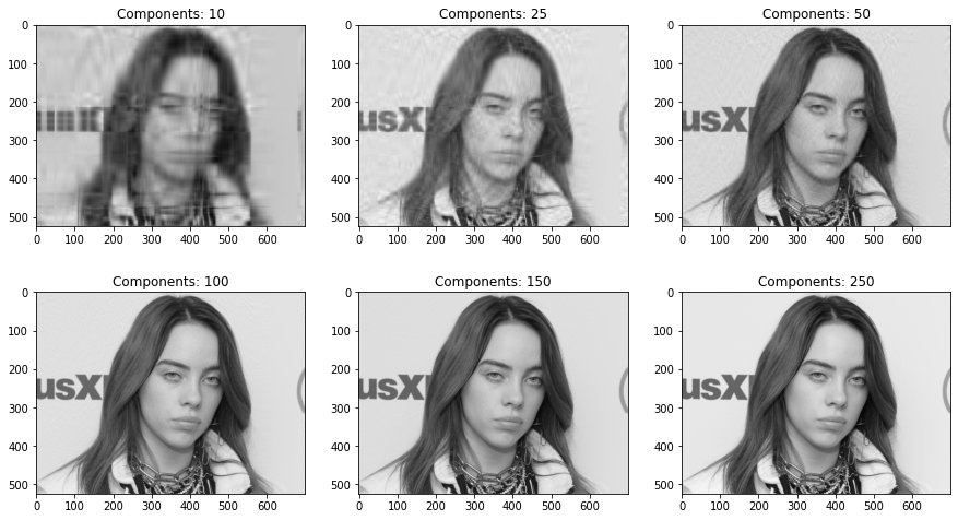
Plotting the same for different numbers of components to compare the exact relative difference,
#setting different amounts of K
ks = [10, 25, 50, 100, 150, 250]

plt.figure(figsize=[15,9])

for i in range(6):
    plt.subplot(2,3,i+1)
    plot_at_k(ks[i])
    plt.title("Components: "+str(ks[i]))

plt.subplots_adjust(wspace=0.2, hspace=0.0)
plt.show()
Using PCA for Image Reconstruction, we can also segregate between the amounts of RGB present in an image,
import cv2
img = cv2.cvtColor(cv2.imread('/content/5d10e5939c5101174c54bb98.png'), cv2.COLOR_BGR2RGB)
plt.imshow(img)
plt.show()

#Splitting into channels
blue,green,red = cv2.split(img)
# Plotting the images
fig = plt.figure(figsize = (15, 7.2))
fig.add_subplot(131)
plt.title("Blue Presence")
plt.imshow(blue)
fig.add_subplot(132)
plt.title("Green Presence")
plt.imshow(green)
fig.add_subplot(133)
plt.title("Red Presence")
plt.imshow(red)
plt.show()

A particular image channel can also be converted into a data frame for further processing,
import numpy as np
import pandas as pd

#creating dataframe from blue presence in image
blue_chnl_df = pd.DataFrame(data=blue)
blue_chnl_df

The data for each color presence can also be fit and transformed to a particular number of components for checking the variance of each color presence,
#scaling data between 0 to 1
df_blue = blue/255
df_green = green/255
df_red = red/255


#setting a reduced number of components
pca_b = PCA(n_components=50)
pca_b.fit(df_blue)
trans_pca_b = pca_b.transform(df_blue)
pca_g = PCA(n_components=50)
pca_g.fit(df_green)
trans_pca_g = pca_g.transform(df_green)
pca_r = PCA(n_components=50)
pca_r.fit(df_red)
trans_pca_r = pca_r.transform(df_red)

#transforming shape
print(trans_pca_b.shape)
print(trans_pca_r.shape)
print(trans_pca_g.shape)


#checking variance after reduced components
print(f"Blue Channel : {sum(pca_b.explained_variance_ratio_)}")
print(f"Green Channel: {sum(pca_g.explained_variance_ratio_)}")
print(f"Red Channel  : {sum(pca_r.explained_variance_ratio_)}")
Output :
Blue Channel : 0.9835704508744926
Green Channel: 0.9794100254497594
Red Channel  : 0.9763416610407115
We can observe that by only using 50 components we can keep around 98% of the variance in the data!
End Notes
In this article, we understood what Principal Component Analysis is and how it can be used for Image Reconstruction and Processing. We also tried hands-on implementation of the PCA features for image processing on a sample image. The above code can be found in a Colab notebook, which can be accessed using the link here.
Happy Learning!


