Deep neural networks learn to form relationships with the given data without having prior exposure to the dataset. They perform very well on non-linear data and hence require large amounts of data for training. Although more information is better for the network, it leads to problems like overfitting. 

The neural network will work really well with training data but underperforms when it is fed unseen data. This makes the network blind to the uncertainties in the training data and tends to be overly confident in its wrong predictions. Consider an example where you are trying to classify a car and a bike. If an image of a truck is shown to the network, it ideally should not predict anything. But, because of the softmax function, it assigns a high probability to one of the classes and the network wrongly, though confidently predicts it to be a car. In order to avoid this, we use the Bayesian Neural Network (BNN).

What will we discuss in this article?

• Why do we need to use BNN?
• How a Bayesian network works
• Implementing a BNN

Why do we need to use the Bayesian Neural Network (BNN)?

As discussed above, we need to make sure our model does not overfit. You may be wondering that there are other methods to do this like Batch Normalisation, Dropout etc. But all these methods do not solve the problem of identifying uncertainty in the model. Hence the need for BNNs. Bayesian Networks work well on small datasets and are robust for avoiding overfitting. They also come with additional features like uncertainty estimation, probability distributions etc.

How Does a Bayesian Neural Network work?

The motto behind a BNN is pretty simple — every entity is associated with a probability distribution, including weights and biases. There are values called ‘random variables’ in the bayesian world which provides a different value every time it is accessed. Let X be a random variable which represents the normal distribution, every time you access X, it’ll have a different value. This process of obtaining a different value on each access is called Sampling. What value comes out of each sample depends on the probability distribution. The wider the probability distribution, the more the uncertainty. 

In a traditional neural network, each layer has fixed weights and biases that determine the output. But, a Bayesian neural network will have a probability distribution attached to each layer as shown below.

For a classification problem, you perform multiple forward passes each time with new samples of weights and biases. There is one output provided for each forward pass. The uncertainty will be high if the input image is something the network has never seen for all output classes. 

Implementation

We will now implement the BNN on a small dataset from sklearn called iris dataset. This dataset has 4 attributes and around 150 data points. 

Loading the dataset and importing essential packages

import numpy as np
from sklearn import datasets
import torch
import torch.nn as nn
import torch.optim as optim
import torchbnn as bnn
import matplotlib.pyplot as plt

dataset = datasets.load_iris()

Splitting the dataset into data and target and converting them to tensors

data = dataset.data
target = dataset.target 
data_tensor=torch.from_numpy(data).float()
target_tensor=torch.from_numpy(target).long()

Defining a simple Bayesian model

model = nn.Sequential(
    bnn.BayesLinear(prior_mu=0, prior_sigma=0.1, in_features=4, out_features=100),
    nn.ReLU(),
    bnn.BayesLinear(prior_mu=0, prior_sigma=0.1, in_features=100, out_features=3),
)

prior_mu (Float) is the mean of prior normal distribution.
prior_sigma (Float) is the sigma of prior normal distribution.

Defining loss function

The two-loss functions used here are cross-entropy loss and the BKL loss which is used to compute the KL (Kullback–Leibler) divergence of the network.

cross_entropy_loss = nn.CrossEntropyLoss()
klloss = bnn.BKLLoss(reduction='mean', last_layer_only=False)
klweight = 0.01
optimizer = optim.Adam(model.parameters(), lr=0.01)

Training the model

The model is trained for 3000 steps(this would have lead to overfitting for a traditional network)

for step in range(3000):
    models = model(data_tensor)
    cross_entropy = cross_entropy_loss(models, target)
    kl = klloss(model)
    total_cost = cross_entropy + klweight*kl

    optimizer.zero_grad()
    total_cost.backward()
    optimizer.step()
  
_, predicted = torch.max(models.data, 1)
final = target_tensor.size(0)
correct = (predicted == target_tensor).sum()
print('- Accuracy: %f %%' % (100 * float(correct) / final))
print('- CE : %2.2f, KL : %2.2f' % (cross_entropy.item(), kl.item()))

Output : - Accuracy: 98.000000 %
- CE : 0.05, KL : 2.81

Visualisation 

Let us now visualise the model and see how it has performed. To understand how sampling works, run the model multiple times and plot the graphs. You will notice minor changes with each iteration.

def draw_graph(predicted) :
    fig = plt.figure(figsize = (16, 8))

    fig_1 = fig.add_subplot(1, 2, 1)
    fig_2 = fig.add_subplot(1, 2, 2)

    z1_plot = fig_1.scatter(data[:, 0], data[:, 1], c = target,marker=’v’)
    z2_plot = fig_2.scatter(data[:, 0], data[:, 1], c = predicted)

    plt.colorbar(z1_plot,ax=fig_1)
    plt.colorbar(z2_plot,ax=fig_2)

    fig_1.set_title("REAL")
    fig_2.set_title("PREDICT")

    plt.show()

Run 1 : 
models = model(data)
_, predicted = torch.max(models.data, 1)
draw_graph(predicted)











Run 2: 
models = model(data)
_, predicted = torch.max(models.data, 1)
draw_graph(predicted)

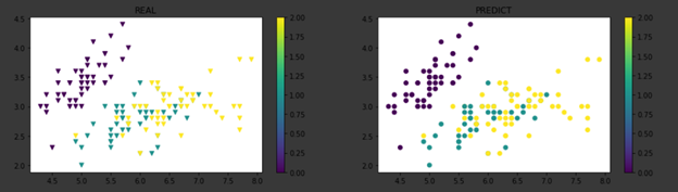
The above graph indicates the difference between the scattering of data points in the actual dataset versus the scattering of points in the predicted bayesian network. Since there are 3 output classes, each of them are indicated in a different color. Each time the data is sampled, the network assigns a probability distribution to the entire input data. On close observation near coordinates (2.3,6.2) of the predicted graph, there is a different prediction made because of the change in probability.

Conclusion

The above implementation makes it clear that not only the problem of overfitting is much more robustly solved with the help of Bayesian Networks but also determines the uncertainty involved in the input.