Hands-on Guide to Image Denoising using Encoder-Decoder Model

Having clear and processed images or videos is very important in any computer vision task. There can be various kinds of unwanted effects and pixels present in images that affect the results of modelling with such images. Noise is also a kind of unwanted information that can harm the information present in the data, so we are required to deal with it. In this article, we are going to see how we can remove noise from the image data using an encoder-decoder model. We will go through two approaches of denoising with encoder-decoder, one with dense layers and one with convolutional layers. The major points to be covered in this article are listed below.

Table of Contents

1. What is Noise?
2. Encoder decoder with Dense layers 
   1. Data preparation 
   2. Model preparation 
   3. Model compiling and training
   4. Model Validation
3. Encoder decoder with convolution layers 
   1. Model preparation 
   2. Model compiling and training
   3. Model Validation

Let us begin the discussion by understanding the noise in images.

What is Noise?

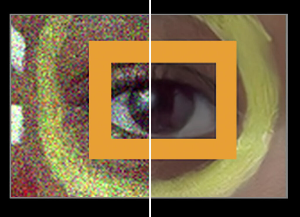
In image data or in a particular image noise can be defined as the pixel values that are in excess in the image and unnecessary. These pixel values are responsible for bad visualization of the image and in many of the tasks they can cause the loss of the information from the image. We can categorize the noise into two types:

• Impulse noise: When pixels of the images are completely different from the pixels which are present in the surrounding in a similar image we can say that the pixels are impulse noise. There can be two types of impulse noise

1. Salt-and-pepper impulse noise (SPIN)
2. Random valued impulse noise (RVIN)

• Additive White Gaussian Noise: This type of noise can be defined as the changes in the overall pixels of the image in a small amount. 

From the above, we can say that the noise is the changes in the pixel values and when the changes occur it can be caused by the loss of information. In such a scenario it becomes very necessary to remove the noise from the images or more simply recover the image from the noise effects. In this article, we will see how we can do the denoising of the images using the neural network.

Denoising by Deep Artificial Neural Network

This type of neural network can be considered as the network for unsupervised learning which can be trained for copying from input to output. When working with the image data this type of network can be used to downsample the image in lower dimension and after downsampling, a similar model resamples the image to its original format. In this context, we can define the work of encoders and decoders in the following way:

• Encoder: In the network, the work of the encoder is to encode the data in its lower dimension of downsampling the data.
• Decoder: The work of the decoder in the network is to upsample the data or make the data of higher dimension from the lower dimension.

The below image is a representation of the work from the encoder-decoder network.

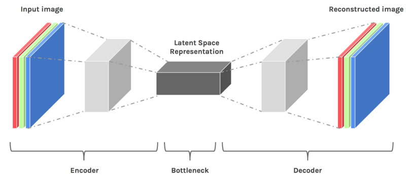
 Image source 

To start this project we are required to import some of the libraries so let’s start the implementation with importing libraries.

Importing libraries: 

import numpy 
import matplotlib.pyplot as plt
import tensorflow as tf
from tensorflow.keras import layers, models
from PIL import ImageFont
import visualkeras

Note: we are using visualkeras library which can be used for visualization of the models made by using Keras and Keras from TensorFlow. For more information about the visualization of neural networks, the reader can go through this article.

Data Preparation 

In the procedure, we will be using the MNIST dataset which is mainly for classification and consists of 60000 images of size 28×28 of 10 digits. More information about the dataset can be read from this link.

Loading the dataset:

(X_train, y_train), (X_test, y_test) = keras.datasets.mnist.load_data()

Since in the procedure we are dealing with the noise of the image so we don’t require the dependent variable of the dataset. Let’s visualize the dataset. 

plt.figure(figsize=(20, 4))
print("Train images")
for i in range(10,20,1):
    plt.subplot(2, 10, i+1)
    plt.imshow(X_train[i,:,:], cmap='gray')
    #plt.title("Test Images with Noise")
plt.show()

Output:

Here we can see the image in the dataset has the digits on the image but we can say that the noise in the image is lower. So we are required to add some pixels to the images so that we can define them as noise.

Also to work with the network we are required to make the dimension of the image in the form of a 2-D array. Before this, we can check the dimension of the data that we are using.

print(X_train.shape)
print(X_test.shape)

Output:

Here we can see that the shape of the dataset is in the form of the 3-D array where 28 x 28 is the image size. To make it a 2-d array we can multiply the second and third dimensions and replace the image size with the multiplication.

num_pixels = 28*28
X_train = X_train.reshape(60000, num_pixels).astype('float32')
X_test = X_test.reshape(10000, num_pixels).astype('float32')

Let’s check for the shape again:

print("train set", X_train.shape)
print("test set", X_test.shape)

Output:

As we have discussed that the noise level is lower so we can add noise to the images using the following lines of codes:

noise_level = 0.5
x_noisy_train = X_train + noise_level * numpy.random.normal(loc=0.0, scale=1.0, size=X_train.shape)
x_noisy_test = X_test + noise_level * numpy.random.normal(loc=0.0, scale=1.0, size=X_test.shape)
x_noisy_train = numpy.clip(x_noisy_train, 0., 1.)
x_noisy_test = numpy.clip(x_noisy_test, 0., 1.)

Let’s check how the images will look like after adding the noise.

x_noisy_train_V = numpy.reshape(x_noisy_train, (-1,28,28)) *255
plt.figure(figsize=(20, 4))
print("Images with Noise")
for i in range(10,20,1):
    plt.subplot(2, 10, i+1)
    plt.imshow(x_noisy_train[i,:,:], cmap='gray')
    plt.title("Image with Noise")
plt.show()

Output:

Here we can see that we have added noise to the images.

Model Preparation 

Now we have images with noise and we can start modelling an encoder-decoder model which can help us in reducing the noise of the images.

# create model
from keras.models import Sequential
from keras.layers import Dense
enco_deco = Sequential()
# Encoder
enco_deco.add(Dense(500, input_dim=num_pixels, activation='relu'))
enco_deco.add(Dense(300, activation='relu'))
enco_deco.add(Dense(300, activation='relu'))
enco_deco.add(Dense(100, activation='relu'))
 
#decoder
enco_deco.add(Dense(300, activation='relu'))
enco_deco.add(Dense(500, activation='relu'))
enco_deco.add(Dense(784, activation='sigmoid'))

Output:

Here in the visualization, we can see how the size of the layers is changing, and somewhere it is similar to the image which we have used in the introduction of the encoder-decoder model.

We can also check it in the summary of the model.

enco_deco.summary()

Output:

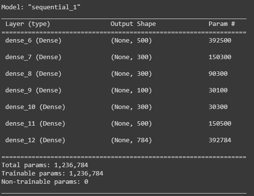
Here we can also see in the parameters that they are changing towards the lower side and again they have increased at the last. As we have discussed in the case of the image the encoder-decoder model first downsample the data and then up-samples the data to match the size of the input.

Model Compiling and Training

Now we can compile and train the models. Here in this example, I am using the adam optimizer and means squared error as the validation loss in the compilation of the model.

# Compile the enco_deco
enco_deco.compile(loss='mean_squared_error', optimizer='adam')

After compiling we can train our model by fitting the data that we have prepared. We are using 5 epochs and a batch size of 200 for training the model.

# Training enco_deco
enco_deco.fit(x_noisy_train, X_train, validation_data=(x_noisy_test, X_test), epochs=5, batch_size=200)

Output:

Model Validation

As we can see that we have trained the model in that section we will look at the workability of the model. By looking at the model training report we can say that losses in the model are lower so we can hope that the model will work fine.

Let’s predict with the test data.

predictions = enco_deco.predict(x_noisy_test)
print("prediction set", predictions.shape)

Output:

Here we can see that the shape of the data is the same but we are required to check on the visualization of the images in the prediction set. We can perform this using the following lines of code.

X_test = numpy.reshape(X_test, (10000,28,28)) *255
plt.figure(figsize=(20, 4))
print("Train images")
for i in range(5,10,1):
    plt.subplot(2, 10, i+1)
    plt.imshow(X_test[i,:,:], cmap='gray')
plt.show()
 
x_test_noisy = numpy.reshape(x_noisy_test, (-1,28,28)) *255
plt.figure(figsize=(20, 4))
for i in range(5,10,1):
    plt.subplot(2, 10, i+1)
    plt.imshow(x_test_noisy[i,:,:], cmap='gray')
    plt.title("Test Images with Noise")
plt.show()    
 
prediction = numpy.reshape(predictions, (10000,28,28)) *255
plt.figure(figsize=(20, 4))
for i in range(5,10,1):
    plt.subplot(2, 10, i+1)
    plt.imshow(prediction[i,:,:], cmap='gray')
    plt.title("recoverd Images")  
plt.show()

Output:

Here we can see all the images from their original to their recovered form. We can also make an encoder-decoder model with convolution and pooling layer lets try this also 

Encoder-Decoder with Convolution Layers 

convolutional layers provide various features to perform different tasks of image processing and using convolutional layers and pooling layers downsample the height and width of the input where transposed convolution layers can be used for upsampling or resampling the data. To know more about the convolutional layer, readers can follow this article.  Let’s start with the implementation of the model consisting of convolution layers. 

Importing the layers:

from tensorflow.keras.models import Model
from keras.layers import Conv2D, Conv2DTranspose, MaxPooling2D

Model preparation 

in_shape = layers.Input(shape=(28, 28, 1))
 
# Encoder
layer = Conv2D(32, (3, 3), activation="relu", padding="same")(in_shape)
layer = MaxPooling2D((2, 2), padding="same")(layer)
layer = Conv2D(32, (3, 3), activation="relu", padding="same")(layer)
layer = MaxPooling2D((2, 2), padding="same")(layer)
 
# Decoder
layer = Conv2DTranspose(32, (3, 3), strides=2, activation="relu", padding="same")(layer)
layer = Conv2DTranspose(32, (3, 3), strides=2, activation="relu", padding="same")(layer)
layer = Conv2D(1, (3, 3), activation="sigmoid", padding="same")(layer)
 
# ecoder decoder
autoencoder = Model(in_shape, layer)

Output:

Here we can see that using the models with convolutional layers we can use more variations in the dimensions. let’s fit the model in the data with noise.

Model Compiling and Training

convomodel.compile(optimizer="adam", loss="binary_crossentropy")

Training the model on noisy data.

convomodel.fit(x_noisy_train, X_train, validation_data=(x_noisy_test, X_test), epochs=5, batch_size=200)

Output:

Model Validation

predictions = convomodel.predict(x_noisy_test)

Checking the shape of the predictions.

print("prediction set", predictions.shape)

Output:

Now we can visualize both of the predictions or recovery images from this approach 

X_test = numpy.reshape(X_test, (10000,28,28)) *255
plt.figure(figsize=(20, 4))
for i in range(5,10,1):
    plt.subplot(2, 10, i+1)
    plt.imshow(X_test[i,:,:], cmap='gray')
    plt.title("original")
plt.show()
 
x_test_noisy = numpy.reshape(x_noisy_test, (-1,28,28)) *255
plt.figure(figsize=(20, 4))
for i in range(5,10,1):
    plt.subplot(2, 10, i+1)
    plt.imshow(x_test_noisy[i,:,:], cmap='gray')
    plt.title("Test Images with Noise")
plt.show()    
 
predict = numpy.reshape(predictions, (10000,28,28)) *255
plt.figure(figsize=(20, 4))
for i in range(5,10,1):
    plt.subplot(2, 10, i+1)
    plt.imshow(predict[i,:,:], cmap='gray')
    plt.title("recoverd Images")  
plt.show()

Output:

Here we can see that we have a clearer image than the first used encoder-decoder layer where all the layers were flattened layers. 

Final Words 

In the article, we have seen an overview of noise along with denoising approaches. We could understand how we can remove noise from the image using the deep neural network, where we have applied two approaches of neural network using dense layers and using convolutional layers. 

References:

• Autoencoder
• Link for the Codes