Every beginner in data science goes through simple projects like diabetes prediction, Market basket analysis, and some basic regression problems. All these projects we have carried out are based on structured data and that too in the tabular format. But this will not be the situation every time; the data in real-time is much more complex. So you have first to collect it from various sources, understand it and arrange it in a format that is ready for processing.
This way is even more difficult when data is in an unstructured format such as Audio, Images, Text, and so on; this is because you can not represent these data in its raw format, which is really hard to interpret; therefore, standard representation way has to be adopted for the better understanding of these data.
By the facts, a very large amount of unstructured data represents huge under-exploited opportunities. For example, if you look at our daily communication, you get what the person wants to say or convey and easily interpret their attitude towards you. So, in short, unstructured data is complex, but with the right tools and proper techniques, we can easily get those insights.
Today, in this article, we will talk about handling audio files, different representation techniques, and decomposing files.
Code Implementation: Librosa
The first step is to load the file into the machine to be readable by them. At this step, we simply take values after every specific time step. For example, for a 30 seconds audio file, we extract values for the 10th second this is called sampling and the rate at which these samples are collected is called the sampling rate.
Proceeding further, below practical implementation shows how to load audio files, how to represent the files in time and frequency domain using various plots, how to do feature extraction like chromogram and tempogram, and lastly, we will see how to do the remix.
Import & install all dependencies:
! pip install librosa
! pip install mir_eval
import librosa
import librosa.display as dsp
import mir_eval
from IPython.display import Audio
import matplotlib.pyplot as plt
import numpy as np
Load the files:
Here we are loading single-channel and two-channel audio files from the librosa audio sample. Single referred as mono in signal domain contains only one channel, and other is stereo which contains multiple channels. You can differentiate between these files easily with your headset; if you hear sound simultaneously at both headsets, it is a single channel file; otherwise, it is multi-channel.
Below I loaded both types of files; you can check the effect.
## mono file
data1, sample_rate = librosa.load(librosa.util.example_audio_file(),duration=60)
Audio(data=data1,rate=sample_rate)
## stereo file
data2, sample_rate = librosa.load(librosa.util.example_audio_file(), mono=False,duration=60)
Audio(data=data2,rate=sample_rate)You can load your own file by specifying the path inside librosa.load()
Let’s check some basic information about file,
print('Total number of samples: ',data1.shape[0])
print('Sample rate: ',sample_rate)
print('Lenngth of file in seconds: ',librosa.get_duration(data1))
The sampling rate is nothing but samples taken per second, and by default, librosa samples the file at a sampling rate of 22050; you can override it by your desired sampling rate. Take the product of sampling rate and length of the file you will get the total number of samples.
If you are dealing with large audio files, this sampling rate is a more concerning factor as it adds a significant amount of load time. For this case, you can define resample type inside load function as like below;
start = time.clock()
data, rate = librosa.load('/content/Electronic-house-background-music-118-bpm.mp3',res_type='kaiser_fast')
after = time.clock()-start
print('Time taken to load file before and after applying resampling type resp: ',before, after)
Visualize the waveplot and spectrogram:
Waveplot:
Wave Plots are used to plot the natural waveform of an audio file for time, and ideally, it is sinusoidal. Here I have plotted the wave plot for both mono and stereotype of the same audio file.
Look closer to the waveform;
plt.plot(data1)
plt.xlim([2000,3000])
fig, ax = plt.subplots(nrows=2, sharex=True,figsize=(10,7))
librosa.display.waveshow(data1, sr=sample_rate, ax=ax[0])
ax[0].set(title='Envelope view, mono')
ax[0].label_outer()
librosa.display.waveshow(data2, sr=sample_rate, ax=ax[1])
ax[1].set(title='Envelope view, stereo')
ax[1].label_outer()
Spectrogram:
The spectrogram is a visual representation of a spectrum of different frequencies for time. Here we are plotting the spectrogram for linear frequencies and log frequencies. The use of these two types of spectrogram completely relies on matters of interest. If you are more interested in higher frequencies than lower ones, you should go with a linear frequencies plot.
d = librosa.stft(data1)
D = librosa.amplitude_to_db(np.abs(d),ref=np.max)
fig,ax = plt.subplots(2,1,sharex=True,figsize=(10,10))
img = dsp.specshow(D, y_axis='linear', x_axis='s',sr=sample_rate,ax=ax[0])
ax[0].set(title='Linear frequency power spectrogram')
ax[0].label_outer()
dsp.specshow(D,y_axis='log',x_axis='s',sr=sample_rate,ax=ax[1])
ax[1].set(title='Log frequency power spectrogram')
ax[1].label_outer()
fig.colorbar(img, ax=ax, format='%+2.f dB')
From the above two spectrograms, we can easily say that the file contains the most information at lower frequencies; both graphs contain the same information. Therefore, to carry out further analysis, we should use a log frequency plot.
Feature Extraction:
Chromagram:
Chromagram closely relates to the twelve different pitch classes; these features are powerful tools for analysing music whose pitches can be meaningfully categorized often into twelve categories. One main property of chroma features is capturing harmonic and melodic characteristics of music while being an extensive change in the timbre and instrumentation.
C = np.abs(librosa.stft(data1))
chroma = librosa.feature.chroma_stft(S=C, sr=sr)
fig, ax = plt.subplots(figsize=(10,6))
img = librosa.display.specshow(chroma, y_axis='chroma', x_axis='s', ax=ax)
fig.colorbar(img, ax=ax)
ax.set(title='Chromagram')
Tempogram:
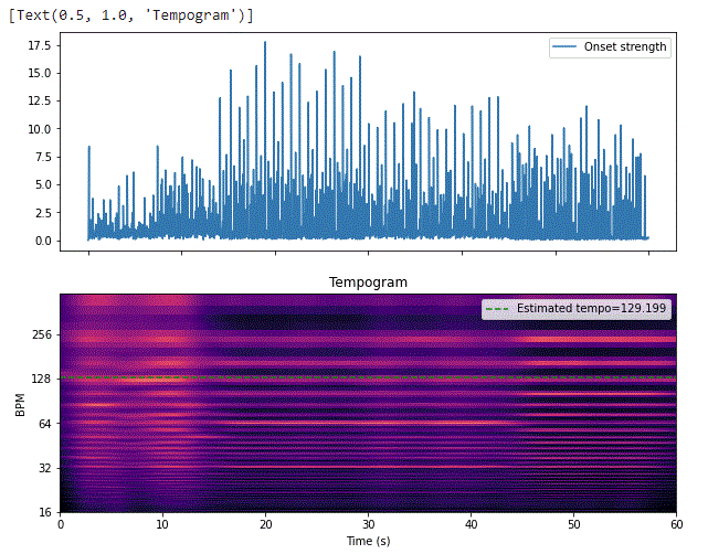
It is a time pulse representation of an audio signal laid out such that it indicates the variation of pulse strength over time, given a specific time lag or BPM value. The construction of a tempogram can be divided into two parts. First, the onset detection characterizes a series of musical events constituting the basic rhythmic content of the audio. This is followed by the estimation of local tempo using the autocorrelation or Fourier transform of the onset detection function computed over a short time window.
For further information regarding these kinds of terminologies, you can refer to this paper.
oenv = librosa.onset.onset_strength(y=data1, sr=sample_rate)
tempogram = librosa.feature.tempogram(onset_envelope=oenv, sr=sample_rate)
# Compute global onset autocorrelation
ac_global = librosa.autocorrelate(oenv, max_size=tempogram.shape[0])
ac_global = librosa.util.normalize(ac_global)
# Estimate the global tempo for display purposes
tempo = librosa.beat.tempo(onset_envelope=oenv, sr=sample_rate)[0]
fig, ax = plt.subplots(nrows=2, figsize=(10, 8))
times = librosa.times_like(oenv, sr=sample_rate)
ax[0].plot(times, oenv, label='Onset strength')
ax[0].label_outer()
ax[0].legend(frameon=True)
librosa.display.specshow(tempogram, sr=sample_rate,x_axis='s',
     y_axis='tempo', cmap='magma',ax=ax[1])
ax[1].axhline(tempo, color='g', linestyle='--', alpha=1,
            label='Estimated tempo={:g}'.format(tempo))
ax[1].legend(loc='upper right')
ax[1].set(title='Tempogram')
Separating the components:
This section will show how to separate the frequencies component like harmonic and percussive component from an audio file, later how to manipulate the audio stream like slowing and fasting the tempo; lastly, we will see how to sonify the click sound with the audio file.
files=librosa.ex('brahms')
y,sr = librosa.load(files)
# separate components
y_harmonic, y_percussive = librosa.effects.hpss(y)
# Original file
Audio(y,rate=sr)# harmonic component
Audio(y_harmonic,rate=sr)# percussive component
Audio(y_percussive,rate=sr)# slowing the tempo
y_slow = librosa.effects.time_stretch(y, 0.7)
Audio(y_slow,rate=sr)By listening to the above files, we can easily differentiate between these frequency components and the tempo effect.
# remixing
tempo, beats = librosa.beat.beat_track(y=y_slow, sr=sr)
beat_times = librosa.frames_to_time(beats)
y_tone = mir_eval.sonify.clicks(beat_times,sr,length=len(y_slow))
Audio(y_slow+y_tone,rate=sr)
Conclusion:
This was all about starting with librosa, where we have seen from loading files to plotting different graphs and manipulating the files. The use of audio features is completely dependent on the type of problem you are dealing with. For example, you are dealing with detecting pitches present in the audio file; in this case, chromogram should be the choice for tasks like these; each feature has a different role and helps to get insights. Here you can see the use of spectrogram to recognize keywords present in the audio clips.


