Hands-On Guide to Multi-Class Classification Using Mobilenet_v2

As computer hardware becomes more and more powerful, it has renewed interest in deep learning. In early 2009, big bang kind of thing happened in the deep learning field as the deep learning neural network first time were trained with Nvidia’s graphics processing units (GPU); after that, Andrew Ng came up with the novel conclusion that GPU’s could increase the speed of deep learning systems by hundreds of times, particular saying GPU’s are well suited for matrix or vector-based calculations.       

Innovation of deep neural networks has given rise to many AI-based applications and overcome the difficulties faced by computer vision-based applications such image classification, object detections etc. and frameworks like Tensorflow, PyTorch, Theano, Keras, MxNet has made these task simpler than ever before. 

As you go deeper and deeper with your neural networks with more layers in short, if you tend to make it complex to ensure model robustness, this can lead to a huge training time that can last up to some weeks. This is where the transfer learning came into the picture, where a particular developed model is reused as the starting point to the other task. 

Nowadays, it is the most popular approach in deep learning where pre-trained models are used as a starting point at computer vision and NLP based tasks; this reduces significant training time and requirement of resources such as high computing machines. This method is quite simple; you just have to choose which pre-trained model is suited for your application, and with minimal code, you can have your high performing classifier. 

Today in this article, we will see an approach that shows how one uses the transfer learning method for classification tasks and how the same pre-trained network can be used for your dataset. 

Download our Mobile App

Implementing Multi-Class Classification Using Mobilenet_v2

We are using a pre-trained model called MobileNet_v2, which is a popular network for image-based classification, and trained on 1000 classes of ImageNet dataset with more than 20 million parameters; let’s see how it works.

Import all dependencies:

import numpy as np
#image handling
import PIL.Image as Image
import matplotlib.pyplot as plt
import tensorflow as tf
import tensorflow_hub as hub
import datetime
import time
# for the evaluation
%load_ext tensorboard

As said earlier, we are using a classifier trained on the ImageNet benchmark dataset. In this section, we are trying to classify random images using MobileNet_v2. First, we will load the module from TensorFlow. All the pre-trained models are subjected to the specific size of the input image, so make sure that you reshape the image as below.

classifier_model ='https://tfhub.dev/google/tf2-preview/mobilenet_v2/classification/4'   
shape = (224,224)
## wrap the model with Sequential model
classifier = tf.keras.Sequential([
    hub.KerasLayer(classifier_model, input_shape = shape + (3,))
])

Load the sample image from the web, which we are going to classify;

sample = tf.keras.utils.get_file('3a3127130afaa005b3c8496b66e25faa.jpg','https://i.pinimg.com/originals/3a/31/27/3a3127130afaa005b3c8496b66e25faa.jpg')
sample = Image.open(sample).resize(shape)
sample

Now scale down all the pixels between 0 to 1 as Neural Networks perform better on scaled values and get the model’s prediction.

sample = np.array(sample)/255.0
results = classifier.predict(sample[np.newaxis, ...])
## to aggregate the prediction as it has probabilities values
## for 1000 classes
predicted_class = tf.math.argmax(results[0],axis=-1)

The above-predicted class returns a coded integer that represents a particular class in the ImageNet dataset for which we have to decode the prediction. Now, this can be simply done by matching this ID with a class file as given below.

labels_path = tf.keras.utils.get_file('ImageNetLabels.txt','https://storage.googleapis.com/download.tensorflow.org/data/ImageNetLabels.txt')
imagenet_labels = np.array(open(labels_path).read().splitlines())

Below is the prediction of our image:

plt.imshow(sample)
plt.axis('off')
predicted_cls_name = imagenet_labels[predicted_class]
plt.title('Prediction: '+ predicted_cls_name.title())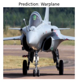

With such minimal code, we have a fairly strong classifier; the transfer learning is not limited up to this; we can also have such a classifier for our dataset. We just need to load data in a proper way such that it can be used for training and have to do some model changes.

Below, we are going to use MobileNet_v2 for the flower dataset, which has five different classes of flowers; now onwards, we are using Keras functional API for further coding.

Load the dataset as below;

root = tf.keras.utils.get_file('flower_photos',      'https://storage.googleapis.com/download.tensorflow.org/example_images/flower_photos.tgz',untar=True)
batch_size = 64
height = 224
width = 224
train_data = tf.keras.preprocessing.image_dataset_from_directory(
    str(root),
    validation_split=0.2,
    seed=123,
    image_size=(height,width),
    batch_size=batch_size
)

vali_data = tf.keras.preprocessing.image_dataset_from_directory(
    str(root),
    validation_split=0.2,
    seed=123,
    image_size = (height,width),
    batch_size=batch_size)

This will return dataset like below;

Below are the classes of our dataset;

classes = np.array(train_data.class_names)
print(classes)

Below are the preprocessing steps that have to be carried out, such as scaling all the images and using buffer prefetching to yield the data without any blocking issues due to I/O ports.   

norm_layer = tf.keras.layers.experimental.preprocessing.Rescaling(1./255)
train_data = train_data.map(lambda x, y: (norm_layer(x), y))
vali_data = vali_data.map(lambda x,y: (norm_layer(x),y))
autotune = tf.data.AUTOTUNE
train_data = train_data.cache().prefetch(buffer_size=autotune)
vali_data = vali_data.cache().prefetch(buffer_size=autotune)

The bottom, top layer of the model has classes of 1000, but we have five classes to predict; Tensorflow also distributes the model without the classification layer, and the last classification layer can be added. Now load the model from TensorFlow and add the last classification layer;

feature_extractor_model = 'https://tfhub.dev/google/tf2-preview/mobilenet_v2/feature_vector/4' 
feature_layer = hub.KerasLayer(
    feature_extractor_model,
    input_shape=(224,224,3),
    trainable=False)
num_classes = len(classes)
model = tf.keras.Sequential([
    feature_layer,
    tf.keras.layers.Dense(num_classes)])
model.summary()

Below is a summary of the model;

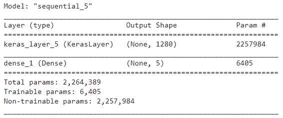
Now compile and train the model;

model.compile(
    optimizer=tf.keras.optimizers.Adam(),
    loss=tf.keras.losses.SparseCategoricalCrossentropy(from_logits=True),
    metrics=['accuracy'])
## store logs for tensorboard
log_dir = 'logs/fit/'+datetime.datetime.now().strftime('%Y%m%d-%H%M%S')
tensorboard_callback = tf.keras.callbacks.TensorBoard(
    log_dir=log_dir,
    histogram_freq=1)

history = model.fit(train_data,validation_data=vali_data,epochs=10,callbacks=tensorboard_callback)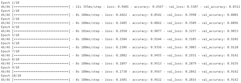

Now check the predictions of our model;

# get and decode the predictions
predicted_batch = model.predict(image)
predicted_id = tf.math.argmax(predicted_batch, axis=-1)
predicted_label = classes[predicted_id]
plt.figure(figsize=(10,7))
plt.subplots_adjust(hspace=0.5)
for i in range(6):
  plt.subplot(2,3,i+1)
  plt.imshow(image[i])
  plt.title(predicted_label[i].title())
  plt.axis('off')
  plt.tight_layout
  plt.suptitle('Model predictions')

Conclusion:

From this article, we have learned how to use a pre-trained model for classification against the 1000 classes of ImageNet dataset and how one can use it for custom datasets such as we have used for flower classifications.   

Reference:

• Link for above codes
• Pre-trained models and dataset