Last updated February 3, 2021
In AI Mysteries

Hands-on Guide to PyTorch 3D – A Library for Deep Learning with 3D Data

Share

Published on February 3, 2021

by Aishwarya Verma

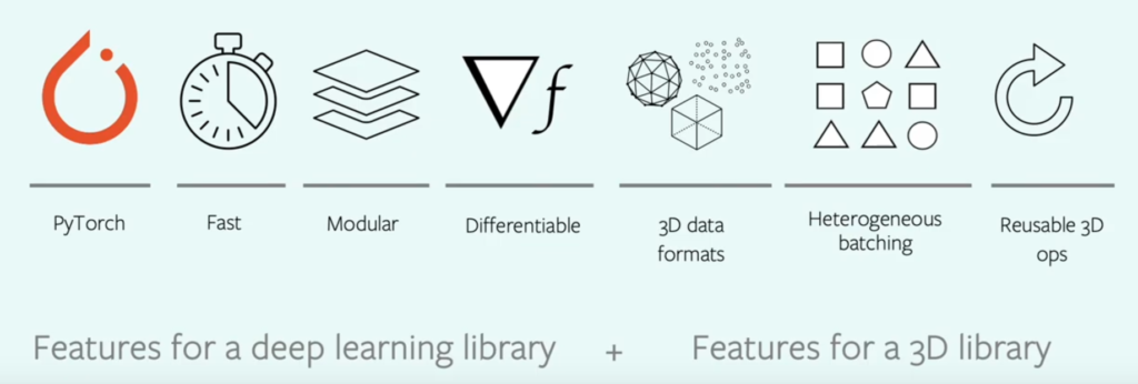
Facebook AI’s PyTorch 3D is a python library to deal with 3D data in deep learning. It is based on PyTorch tensors and highly modular, flexible, efficient and optimized framework, which makes it easier for researchers to experiment with and impart scalability to big 3D data. PyTorch 3D framework contains a set of 3D operators, batching techniques and loss functions(for 3D data) that can be easily integrated with existing deep learning systems through its fast and differentiable API’s. The key features of PyTorch 3D are as follows:

Operations of PyTorch 3D are implemented using PyTorch tensors.
Provides the functionality to use GPU for acceleration.
PyTorch 3D is capable of handling mini-batches of heterogeneous data

You can cover the theoretical aspect of PyTorch 3D through our previous article on PyTorch 3D. In this article, we will cover some Python demos of PyTorch 3D.

Core Components in CodeBase

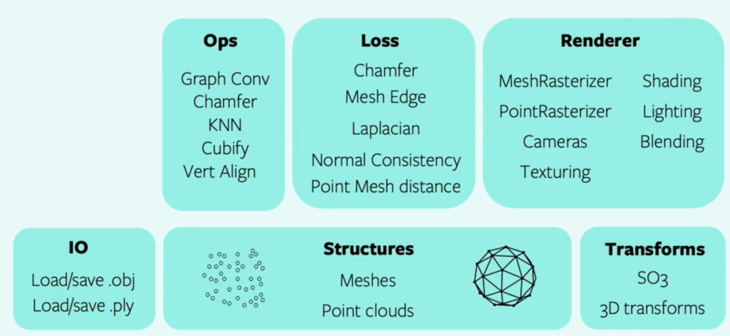
Overview of components in the codebase is shown below. The foundation layer consists of data structures for 3D data, data loading utilities and composable transforms. The data structures in particular enable the operators and loss functions in the second layer to efficiently support heterogeneous batching.

Installation

Install PyTorch 3D through these commands below:

import os
!curl -LO https://github.com/NVIDIA/cub/archive/1.10.0.tar.gz
!tar xzf 1.10.0.tar.gz
#create a new environement
os.environ["CUB_HOME"] = os.getcwd() + "/cub-1.10.0"
!pip install 'git+https://github.com/facebookresearch/pytorch3d.git@stable'

Demo – Deform source mesh to target mesh

In this demo, we will deform an initial generic shape to fit or convert it to a target. It is divided into four parts mainly:

Import all the required packages and libraries. The code snippet is available here. Now, download the target object and save it locally.

!wget https://dl.fbaipublicfiles.com/pytorch3d/data/dolphin/dolphin.obj
# Load the dolphin mesh.
trg_obj = os.path.join('dolphin.obj')

Now, load the target image as an object via load_obj. It will give you tensors of vertices(verts), faces(vertex indices) and aux. Then normalize the tensor of the vertex-indices of each of the corners of the face and then create a mesh with the help of Meshes data structure available in PyTorch 3D.

# We read the target 3D model using load_obj
#which sets verts to be a (V,3)-tensor of vertices and faces.verts_idx to be an (F,3)- tensor of the vertex-indices of each of the corners of 
#the faces. Faces which are not triangles will be split into triangles. aux is an object which may contain normals, 
#uv coordinates, material colors and textures if they are present, and faces may additionally contain indices into these normals, 
#textures and materials in its NamedTuple structure. 
verts, faces, aux = load_obj(trg_obj)

# verts is a FloatTensor of shape (V, 3) where V is the number of vertices in the mesh
# faces is an object which contains the following LongTensors: verts_idx, normals_idx and textures_idx
# For this tutorial, normals and textures are ignored.
faces_idx = faces.verts_idx.to(device)
verts = verts.to(device)

# We scale normalize and center the target mesh to fit in a sphere of radius 1 centered at (0,0,0). 
# (scale, center) will be used to bring the predicted mesh to its original center and scale
# Note that normalizing the target mesh, speeds up the optimization but is not necessary!
center = verts.mean(0)
verts = verts - center
scale = max(verts.abs().max(0)[0])
verts = verts / scale

# We construct a Meshes structure for the target mesh
#initialize a PyTorch3D datastructure called Meshes, 
trg_mesh = Meshes(verts=[verts], faces=[faces_idx])

Now, initialize a source shape to be sphere of radius 1.

# We initialize the source shape to be a sphere of radius 1

#ico_sphere creates verts and faces for a unit ico-sphere, with all faces oriented consistently.
# here, integer specifying the number of iterations for subdivision of the mesh faces. 
#Each additional level will result in four new faces per face.
src_mesh = ico_sphere(4, device)

Now, visualize the source and target mesh. The code snippet is available here.
Now, create a deform_verts of size of source mesh with values 0. We will now deform the mesh by offsetting its vertices.

# We will learn to deform the source mesh by offsetting its vertices
# The shape of the deform parameters is equal to the total number of vertices in src_mesh
verts_shape = src_mesh.verts_packed().shape
#Creates a tensor of size size filled with fill_value= 0.0
deform_verts = torch.full(verts_shape, 0.0, device=device, requires_grad=True)

Then, initialize a stochastic gradient descent as an optimizer.

# The optimizer
#create a stochastic gradient optimizer for the deform_verts with
#learning rate of 1.0
optimizer = torch.optim.SGD([deform_verts], lr=1.0, momentum=0.9)

Now, we will run a loop to learn the offset to each vertex in the mesh so that the predicted mesh is closer to target mesh at each optimization step. The loss function used here are as follows:

chamfer_distance, the distance between the predicted (deformed) and target mesh, defined as an evaluation metric for two point clouds. It takes the distance of each point into account. For each point in each cloud, chamfer_distance finds the nearest point in the other point set and sums the square of distance up.

However, minimizing only the chamfer distance between the predicted and the target mesh will lead to a non-smooth shape. Hence, we will consider other minimization functions i.e., add shape regularizers to the object for smoothness.

mesh_edge_length, which minimizes the length of the edges in the predicted mesh.
mesh_normal_consistency, which enforces consistency across the normals of neighbouring faces.
mesh_laplacian_smoothing, which is the laplacian regularizer.

Initialize the number of iterations and weight of each loss function and then start a loop.

# Number of optimization steps
Niter = 2000
# Weight for the chamfer loss
w_chamfer = 1.0 
# Weight for mesh edge loss
w_edge = 1.0 
# Weight for mesh normal consistency
w_normal = 0.01 
# Weight for mesh laplacian smoothing
w_laplacian = 0.1 
# Plot period for the losses
plot_period = 250

Now, start the loop by initializing the optimizer and offset the verts of deform_verts, to get a new source mesh. Next, sample 5000 each from both new source and target mesh and calculate all the loss functions and create a final loss by giving weights to each loss function. This process will repeat at each iteration. At last, calculate the loss gradient and update the parameters, as shown below in the code.

for i in loop:
    # Initialize optimizer
    optimizer.zero_grad()
    
    # Deform the mesh
    new_src_mesh = src_mesh.offset_verts(deform_verts)
    
    # We sample 5k points from the surface of each mesh 
    sample_trg = sample_points_from_meshes(trg_mesh, 5000)
    sample_src = sample_points_from_meshes(new_src_mesh, 5000)
    
    # We compare the two sets of pointclouds by computing (a) the chamfer loss
    loss_chamfer, _ = chamfer_distance(sample_trg, sample_src)
    
    # and (b) the edge length of the predicted mesh
    loss_edge = mesh_edge_loss(new_src_mesh)
    
    # mesh normal consistency
    loss_normal = mesh_normal_consistency(new_src_mesh)
    
    # mesh laplacian smoothing
    loss_laplacian = mesh_laplacian_smoothing(new_src_mesh, method="uniform")
    
    # Weighted sum of the losses
    loss = loss_chamfer * w_chamfer + loss_edge * w_edge + loss_normal * w_normal + loss_laplacian * w_laplacian
    
    # Print the losses
    loop.set_description('total_loss = %.6f' % loss)
    
    # Save the losses for plotting
    chamfer_losses.append(loss_chamfer)
    edge_losses.append(loss_edge)
    normal_losses.append(loss_normal)
    laplacian_losses.append(loss_laplacian)
    
    # Plot mesh
    if i % plot_period == 0:
        plot_pointcloud(new_src_mesh, title="iter: %d" % i)
        
    # Optimization step
    loss.backward()
    optimizer.step()

The output at each 250 iterations is shown below.

Visualize all the loss functions with respect to the number of iterations.

You can check the full demo here.

Demo – Bundle Adjustments

Bundle Adjustments is state estimation technique used to estimate the location of points in the environment and those points have been estimated from camera images and we do not only want to estimate the location of those points in the world, but we also want to estimate where the camera was, when taking the image and where it was looking. In all, we want to estimate the location of points and camera jointly so the re-projection error where the points are actually projected to, can be minimized. This same problem can be visualized as :

The picture below depicts the situation at the beginning of our optimization. The ground truth cameras are plotted in purple while the randomly initialized estimated cameras are plotted in orange:

We seek to align the estimated (orange) cameras with the ground truth (purple) cameras, by minimizing the difference between pairs of relative cameras. Thus, the solution to the problem should look as follows:

Mathematically, the above problem can be defined by minimizing the Sum of Squared Re-projection Errors

where,

g₁, g₂, . . ., g_N are the extrinsics(location in the world) of N cameras.

g_ij are the set of relative positions that map between coordinate frames of randomly selected pairs of cameras ( i, j ).

d(g_i, g_j) are is a suitable metric that compares the extrinsics of cameras g_i and g_j.

In this demo, we will learn to initialize a batch of Structure from Motion(SfM), setting up loss functions for bundle adjustments and run an optimization loop using Cameras, transforms and so3 API of PyTorch 3D. The steps are as follows:

Import all the required libraries and packages. The code snippet is available here.
Fetch all the utility python script for plotting and SE3 graph of camera. The code snippet for this, is available here.
In practice, the camera extrinsic g_ij and g_i are represented using objects from the SfMPerspectiveCameras class initialized with the corresponding rotation and translation matrices R_absolute and T_absolute that define the extrinsic parameters g = (R, T); R ∈ SO(3); T∈ R³. In order to ensure that R_absolute is a valid rotation matrix, we represent it using an exponential map (implemented with so3_exponential_map) of the axis-angle representation of the rotation log_R_absolute. The code shown below, load the data(camera data) and load the ground truth and relative positions.

# load the SE3 graph of relative/absolute camera positions
camera_graph_file = './data/camera_graph.pth'
(R_absolute_gt, T_absolute_gt), \
    (R_relative, T_relative), \
    relative_edges = \
        torch.load(camera_graph_file)

# create the relative cameras
cameras_relative = SfMPerspectiveCameras(
    R = R_relative.to(device),
    T = T_relative.to(device),
    device = device,
)

# create the absolute ground truth cameras
cameras_absolute_gt = SfMPerspectiveCameras(
    R = R_absolute_gt.to(device),
    T = T_absolute_gt.to(device),
    device = device,
)

# the number of absolute camera positions
N = R_absolute_gt.shape[0]

Next, we will define the optimization functions for calculating camera distance and getting the relative camera. The two functions are :

calc_camera_distance compares a pair of cameras. This function is important as it defines the loss that we are minimizing. The method utilizes the so3_relative_angle function from the SO3 API.

get_relative_camera computes the parameters of a relative camera that maps between a pair of absolute cameras. Here we utilize the compose and inverse class methods from the PyTorch3D Transforms API.

The code for it is shown below:

def calc_camera_distance(cam_1, cam_2):
    """
    Calculates the divergence of a batch of pairs of cameras cam_1, cam_2.
    The distance is composed of the cosine of the relative angle between 
    the rotation components of the camera extrinsics and the l2 distance
    between the translation vectors.
    """
    # rotation distance
    R_distance = (1.-so3_relative_angle(cam_1.R, cam_2.R, cos_angle=True)).mean()
    # translation distance
    T_distance = ((cam_1.T - cam_2.T)**2).sum(1).mean()
    # the final distance is the sum
    return R_distance + T_distance

def get_relative_camera(cams, edges):
    """
    For each pair of indices (i,j) in "edges" generate a camera
    that maps from the coordinates of the camera cams[i] to 
    the coordinates of the camera cams[j]
    """

    # first generate the world-to-view Transform3d objects of each 
    # camera pair (i, j) according to the edges argument
    trans_i, trans_j = [
        SfMPerspectiveCameras(
            R = cams.R[edges[:, i]],
            T = cams.T[edges[:, i]],
            device = device,
        ).get_world_to_view_transform()
         for i in (0, 1)
    ]
    
    # compose the relative transformation as g_i^{-1} g_j
    trans_rel = trans_i.inverse().compose(trans_j)
    
    # generate a camera from the relative transform
    matrix_rel = trans_rel.get_matrix()
    cams_relative = SfMPerspectiveCameras(
                        R = matrix_rel[:, :3, :3],
                        T = matrix_rel[:, 3, :3],
                        device = device,
                    )
    return cams_relative

Now, start the optimization of absolute cameras. We are going to use a Stochastic Gradient Descent optimizer with momentum and we are going to optimize over T_absolute and log_R_absolute. The code is shown below for this process.

# init the optimizer
optimizer = torch.optim.SGD([log_R_absolute, T_absolute], lr=.1, momentum=0.9)

# run the optimization
n_iter = 2000  # fix the number of iterations
for it in range(n_iter):
    # re-init the optimizer gradients
    optimizer.zero_grad()

    # compute the absolute camera rotations as 
    # an exponential map of the logarithms (=axis-angles)
    # of the absolute rotations
    R_absolute = so3_exponential_map(log_R_absolute * camera_mask)

    # get the current absolute cameras
    cameras_absolute = SfMPerspectiveCameras(
        R = R_absolute,
        T = T_absolute * camera_mask,
        device = device,
    )

    # compute the relative cameras as a compositon of the absolute cameras
    cameras_relative_composed = \
        get_relative_camera(cameras_absolute, relative_edges)

    # compare the composed cameras with the ground truth relative cameras
    # camera_distance corresponds to $d$ from the description
    camera_distance = \
        calc_camera_distance(cameras_relative_composed, cameras_relative)

    # our loss function is the camera_distance
    camera_distance.backward()
    
    # apply the gradients
    optimizer.step()

    # plot and print status message
    if it % 200==0 or it==n_iter-1:
        status = 'iteration=%3d; camera_distance=%1.3e' % (it, camera_distance)
        plot_camera_scene(cameras_absolute, cameras_absolute_gt, status)

print('Optimization finished.')

You can check the full demo, here.

Conclusion

In this article, we have talked about PyTorch 3D and its demo for using Mesh data structure – converting deform source mesh to target mesh and also seen the optimized bundle adjustments. The following demo are available at:

You can check other libraries dealing with 3D data, here.

Codes, Docs and Tutorials are available at:

Access all our open Survey & Awards Nomination forms in one place