


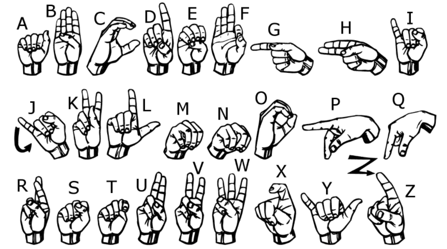
Computer Vision has many interesting applications ranging from industrial applications to social applications. It has also been applied in many support for physically challenged people. For deaf-mute people, computer vision can generate English alphabets based on the sign language symbols. It can recognize the hand symbols and predict the correct corresponding alphabet through sign language classification.
In this article, we will classify the sign language symbols using the Convolutional Neural Network (CNN). After successful training of the CNN model, the corresponding alphabet of a sign language symbol will be predicted. We will evaluate the classification performance of our model using the non-normalized and normalized confusion matrices. Finally, we will obtain the classification accuracy score of the CNN model in this task.
The Data Set
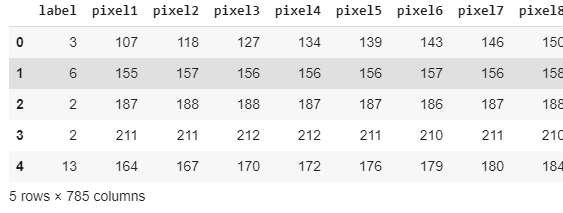
In this article, we have used the American Sign Language (ASL) data set that is provided by MNIST and it is publicly available at Kaggle. This dataset contains 27455 training images and 7172 test images all with a shape of 28 x 28 pixels. These images belong to the 25 classes of English alphabet starting from A to Y (No class labels for Z because of gesture motions). The dataset on Kaggle is available in the CSV format where training data has 27455 rows and 785 columns. The first column of the dataset represents the class label of the image and the remaining 784 columns represent the 28 x 28 pixels. The same paradigm is followed by the test data set.
Implementation of Sign Language Classification
This code was implemented in Google Colab and the .py file was downloaded.
# -*- coding: utf-8 -*-
"""SignLang.ipynb

Automatically generated by Colaboratory.

Original file is located at
    https://colab.research.google.com/drive/1HOyp2uQyxxxxxxxxxxxxxxx
"""
The training and test CSV files were uploaded to the google drive and the drive was mounted with the Colab notebook. The below code snippet are used for that purpose.
#Setting google drive as a directory for dataset
from google.colab import drive
drive.mount('/content/gdrive')
The directory of the uploaded CSV files is defined using the below line of code.
dir_path = "gdrive/My Drive/Dataset"
We will verify the contents of the directory using the below lines of codes.
import os
for dirname, _, filenames in os.walk(dir_path):
    for filename in filenames:
        print(os.path.join(dirname, filename))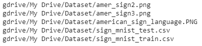
We will print the Sign Language image that we can see in the above list of files.
from IPython.display import Image
Image('gdrive/My Drive/Dataset/amer_sign2.png')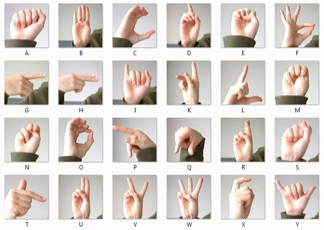
Some important libraries will be uploaded to read the dataset, preprocessing and visualization.
import pandas as pd
import numpy as np
import random
import matplotlib.pyplot as plt
We will read the training and test CSV files
train = pd.read_csv('gdrive/My Drive/Dataset/sign_mnist_train.csv')
test = pd.read_csv('gdrive/My Drive/Dataset/sign_mnist_test.csv')
We will check the shape of the training and test data that we have read above.
print(train.shape)
print(test.shape)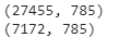
We will check the training data to verify class labels and columns representing pixels.
train.head()
For further preprocessing and visualization, we will convert the data frames into arrays.
# Create training and testing arrays
train_set = np.array(train, dtype = 'float32')
test_set = np.array(test, dtype='float32')
We will specify the class labels for the images.
#Specifying class labels
class_names = ['A', 'B', 'C', 'D', 'E', 'F', 'G', 'H', 'I', 'J', 'K', 'L', 'M', 'N', 'O', 'P', 'Q', 'R', 'S', 'T', 'U', 'V', 'W', 'X', 'Y' ]
We will check a random image from the training set to verify its class label.
#See a random image for class label verification
i = random.randint(1,27455)
plt.imshow(train_set[i,1:].reshape((28,28)))
plt.imshow(train_set[i,1:].reshape((28,28)))
label_index = train["label"][i]
plt.title(f"{class_names[label_index]}")
plt.axis('off')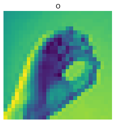
Now, we will plot some random images from the training set with their class labels.
# Define the dimensions of the plot grid
W_grid = 5
L_grid = 5
fig, axes = plt.subplots(L_grid, W_grid, figsize = (10,10))
axes = axes.ravel() # flaten the 15 x 15 matrix into 225 array
n_train = len(train_set) # get the length of the train dataset
# Select a random number from 0 to n_train
for i in np.arange(0, W_grid * L_grid): # create evenly spaces variables
    # Select a random number
    index = np.random.randint(0, n_train)
    # read and display an image with the selected index
    axes[i].imshow( train_set[index,1:].reshape((28,28)) )
    label_index = int(train_set[index,0])
    axes[i].set_title(class_names[label_index], fontsize = 8)
    axes[i].axis('off')
plt.subplots_adjust(hspace=0.4)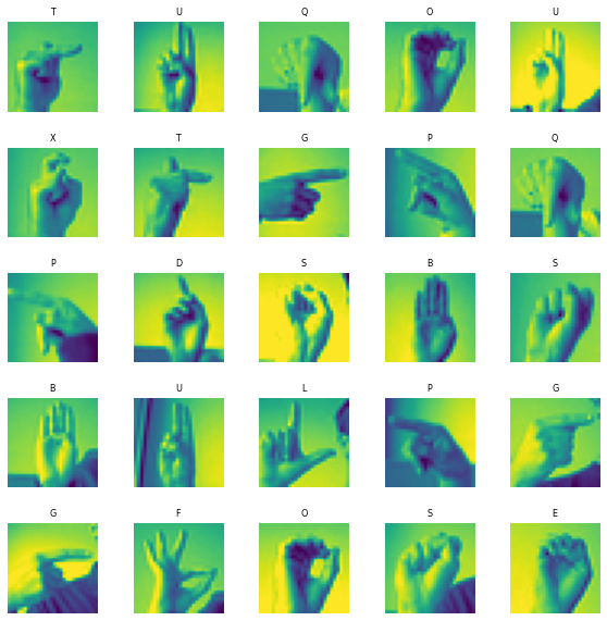
In the next step, we will preprocess out datasets to make them available for the training.
# Prepare the training and testing dataset
X_train = train_set[:, 1:] / 255
y_train = train_set[:, 0]

X_test = test_set[:, 1:] / 255
y_test = test_set[:,0]
From the processed training data, we will plot some random images.
#Visualize train images
plt.figure(figsize=(10, 10))
for i in range(25):
    plt.subplot(5, 5, i + 1)
    plt.xticks([])
    plt.yticks([])
    plt.grid(False)
    plt.imshow(X_train[i].reshape((28,28)), cmap=plt.cm.binary)
    label_index = int(y_train[i])
    plt.title(class_names[label_index])
plt.show()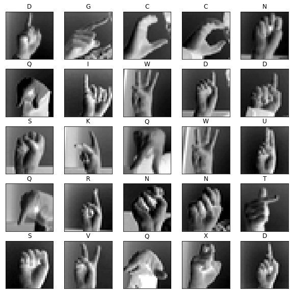
Now, to train the model, we will split our data set into training and test sets.
#Split the training and test sets
from sklearn.model_selection import train_test_split
X_train, X_validate, y_train, y_validate = train_test_split(X_train, y_train, test_size = 0.2, random_state = 12345)
Now, we will check the shape of the training data set.
print(X_train.shape)
print(y_train.shape)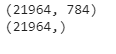
To train the model, we will unfold the data to make it available for training, testing and validation purposes.
# Unpack the training and test tuple
X_train = X_train.reshape(X_train.shape[0], *(28, 28, 1))
X_test = X_test.reshape(X_test.shape[0], *(28, 28, 1))
X_validate = X_validate.reshape(X_validate.shape[0], *(28, 28, 1))

print(X_train.shape)
print(y_train.shape)
print(X_validate.shape)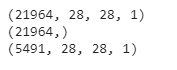
Convolutional Neural Network
In the next step, we will define our Convolutional Neural Network (CNN) Model. For this purpose, first, we will import the required libraries. Make sure that you have installed the TensorFlow if you are working on your local system.
#Library for CNN Model
import keras
from keras.models import Sequential
from keras.layers import Conv2D, MaxPooling2D, Dense, Flatten, Dropout
from keras.optimizers import Adam
from keras.callbacks import TensorBoard

#Defining the Convolutional Neural Network
cnn_model = Sequential()

cnn_model.add(Conv2D(32, (3, 3), input_shape = (28,28,1), activation='relu'))
cnn_model.add(MaxPooling2D(pool_size = (2, 2)))
cnn_model.add(Dropout(0.25))

cnn_model.add(Conv2D(64, (3, 3), input_shape = (28,28,1), activation='relu'))
cnn_model.add(MaxPooling2D(pool_size = (2, 2)))
cnn_model.add(Dropout(0.25))

cnn_model.add(Conv2D(128, (3, 3), input_shape = (28,28,1), activation='relu'))
cnn_model.add(MaxPooling2D(pool_size = (2, 2)))
cnn_model.add(Dropout(0.25))

cnn_model.add(Flatten())

cnn_model.add(Dense(units = 512, activation = 'relu'))
cnn_model.add(Dropout(0.25))
cnn_model.add(Dense(units = 25, activation = 'softmax'))
After defining our model, we will check the model by its summary.
#CNN Model Summary
cnn_model.summary()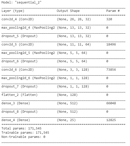
In the next step, we will compile and train the CNN model.
#Compiling
cnn_model.compile(loss ='sparse_categorical_crossentropy', optimizer='adam' ,metrics =['accuracy'])

#Training the CNN model
history = cnn_model.fit(X_train, y_train, batch_size = 512, epochs = 50, verbose = 1, validation_data = (X_validate, y_validate))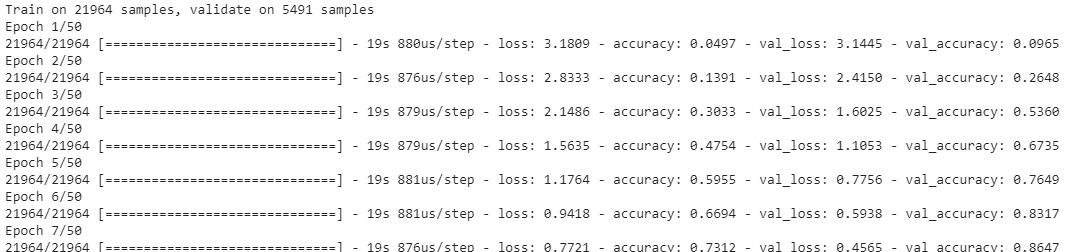

After successful training, we will visualize the training performance of the CNN model.
#Visualizing the training performance
plt.figure(figsize=(12, 8))

plt.subplot(2, 2, 1)
plt.plot(history.history['loss'], label='Loss')
plt.plot(history.history['val_loss'], label='val_Loss')
plt.legend()
plt.grid()
plt.title('Loss evolution')

plt.subplot(2, 2, 2)
plt.plot(history.history['accuracy'], label='accuracy')
plt.plot(history.history['val_accuracy'], label='val_accuracy')
plt.legend()
plt.grid()
plt.title('Accuracy evolution')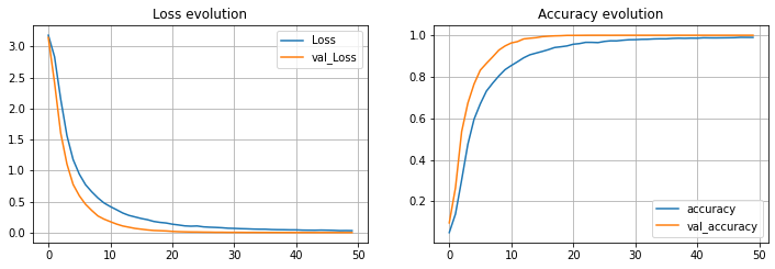
Once we find the training satisfactory, we will use our trained CNN model to make predictions on the unseen test data.
#Predictions for the test data
predicted_classes = cnn_model.predict_classes(X_test)
The CNN model has predicted the class labels for the test images. These predictions will be visualized through a random plot.
#Visualize predictions
L = 5
W = 5

fig, axes = plt.subplots(L, W, figsize = (12,12))
axes = axes.ravel()

for i in np.arange(0, L * W):
    axes[i].imshow(X_test[i].reshape(28,28))
    axes[i].set_title(f"Prediction Class = {predicted_classes[i]:0.1f}\n True Class = {y_test[i]:0.1f}")
    axes[i].axis('off')
plt.subplots_adjust(wspace=0.5)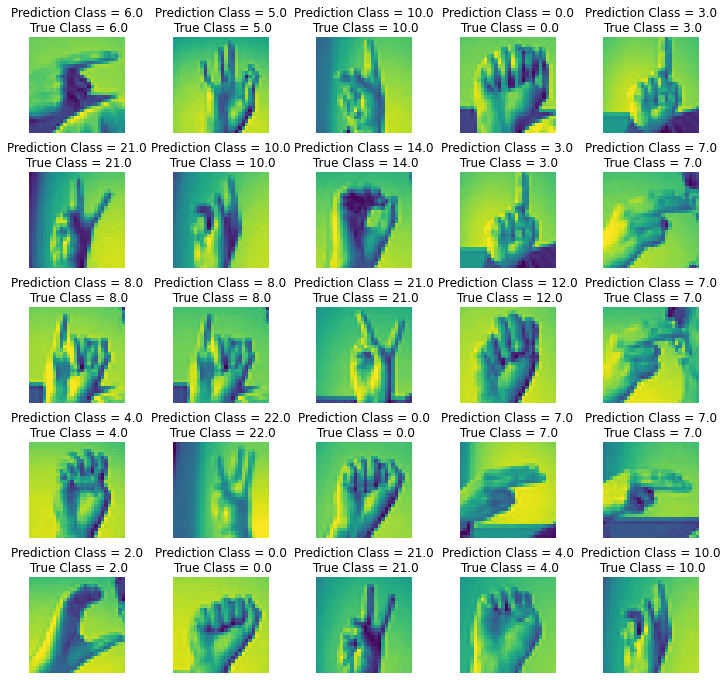
As we can see in the above visualization, the CNN model has predicted the correct class labels for almost all the images. Now we will see the full classification report using a normalized and non-normalized confusion matrices.
from sklearn.metrics import confusion_matrix
from sklearn import metrics
cm = metrics.confusion_matrix(y_test, predicted_classes)
We will define a function to plot the confusion matrix
#Defining function for confusion matrix plot
def plot_confusion_matrix(y_true, y_pred, classes,
                          normalize=False,
                          title=None,
                          cmap=plt.cm.Blues):
    if not title:
        if normalize:
            title = 'Normalized confusion matrix'
        else:
            title = 'Confusion matrix, without normalization'

    # Computing confusion matrix
    cm = confusion_matrix(y_true, y_pred)
    if normalize:
        cm = cm.astype('float') / cm.sum(axis=1)[:, np.newaxis]
        print("Normalized confusion matrix")
    else:
        print('Confusion matrix, without normalization')

# Visualizing
    fig, ax = plt.subplots(figsize=(10, 10))
    im = ax.imshow(cm, interpolation='nearest', cmap=cmap)
    ax.figure.colorbar(im, ax=ax)
    # We want to show all ticks...
    ax.set(xticks=np.arange(cm.shape[1]),
           yticks=np.arange(cm.shape[0]),
           xticklabels=classes, yticklabels=classes,
           title=title,
           ylabel='True label',
           xlabel='Predicted label')

   # Rotating the tick labels and setting their alignment.
    plt.setp(ax.get_xticklabels(), rotation=45, ha="right",
             rotation_mode="anchor")
    # Looping over data dimensions and create text annotations.
    fmt = '.2f' if normalize else 'd'
    thresh = cm.max() / 2.
    for i in range(cm.shape[0]):
        for j in range(cm.shape[1]):
            ax.text(j, i, format(cm[i, j], fmt),
                    ha="center", va="center",
                    color="white" if cm[i, j] > thresh else "black")
    fig.tight_layout()
    return ax
np.set_printoptions(precision=2)
Before plotting the confusion matrix, we will specify the class labels.
#Specifying class labels
class_names = ['A', 'B', 'C', 'D', 'E', 'F', 'G', 'H', 'I', 'J', 'K', 'L', 'M', 'N', 'O', 'P', 'Q', 'R', 'S', 'T', 'U', 'V', 'W', 'X', 'Y' ]
#Non-Normalized Confusion Matrix plt.figure(figsize=(20,20)) plot_confusion_matrix(y_test, predicted_classes, classes = class_names, title='Non-Normalized Confusion matrix') plt.show()#Normalized Confusion Matrix plt.figure(figsize=(35,35)) plot_confusion_matrix(y_test, predicted_classes, classes = class_names, normalize=True, title='Non-Normalized Confusion matrix') plt.show()
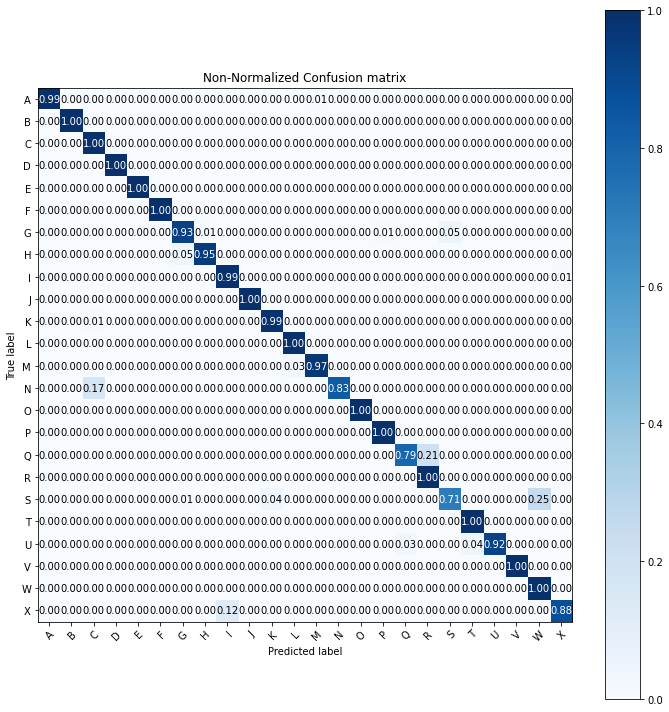
The CNN model has given 100% accuracy in class label prediction for 12 classes, as we can see in the above figure. Now, we will obtain the average classification accuracy score.
#Classification accuracy
from sklearn.metrics import accuracy_score
acc_score = accuracy_score(y_test, predicted_classes)
print('Accuracy Score = ',acc_score)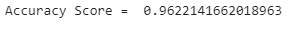
Here, we can conclude that the Convolutional Neural Network has given an outstanding performance in the classification of sign language symbol images. The average accuracy score of the model is more than 96% and it can further be improved by tuning the hyperparameters. We have trained our model in 50 epochs and the accuracy may be improved if we have more epochs of training. However, more than 96% accuracy is also an achievement.