How is Maximum Likelihood Estimation used in machine learning?

Maximum Likelihood Estimation (MLE) is a probabilistic based approach to determine values for the parameters of the model. Parameters could be defined as blueprints for the model because based on that the algorithm works. MLE is a widely used technique in machine learning, time series, panel data and discrete data. The motive of MLE is to maximize the likelihood of values for the parameter to get the desired outcomes. Following are the topics to be covered.

Table of contents

1. What is the likelihood?
2. Working of Maximum Likelihood Estimation
3. Maximum likelihood estimation in machine learning

To understand the concept of Maximum Likelihood Estimation (MLE) you need to understand the concept of Likelihood first and how it is related to probability.

What is the likelihood?

The likelihood function measures the extent to which the data provide support for different values of the parameter. It indicates how likely it is that a particular population will produce a sample. For example, if we compare the likelihood function at two-parameter points and find that for the first parameter the likelihood is greater than the other it could be interpreted as the first parameter being a more plausible value for the learner than the second parameter. More likely it could be said that it uses a hypothesis for concluding the result. Both frequentist and Bayesian analyses consider the likelihood function. The likelihood function is different from the probability density function.

Difference between likelihood and probability density function

Likelihood describes how to find the best distribution of the data for some feature or some situation in the data given a certain value of some feature or situation, while probability describes how to find the chance of something given a sample distribution of data. Let’s understand the difference between the likelihood and probability density function with the help of an example.

Consider a dataset containing the weight of the customers. Let’s say the mean of the data is 70 & the standard deviation is 2.5.

When Probability has to be calculated for any situation using this dataset, then the mean and standard deviation of the dataset will be constant. Let’s say the probability of weight > 70 kg has to be calculated for a random record in the dataset, then the equation will contain weight, mean and standard deviation. Considering the same dataset, now if we need to calculate the probability of weight > 100 kg, then only the height part of the equation be changed and the rest would be unchanged.

But in the case of Likelihood, the equation of the conditional probability flips as compared to the equation in the probability calculation i.e mean and standard deviation of the dataset will be varied to get the maximum likelihood for weight > 70 kg.

Are you looking for a complete repository of Python libraries used in data science, check out here.

Working of Maximum Likelihood Estimation

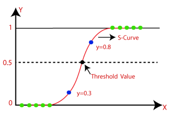
The maximization of the likelihood estimation is the main objective of the MLE. Let’s understand this with an example. Consider there is a binary classification problem in which we need to classify the data into two categories either 0 or 1 based on a feature called “salary”. 

So MLE will calculate the possibility for each data point in salary and then by using that possibility, it will calculate the likelihood of those data points to classify them as either  0 or 1. It will repeat this process of likelihood until the learner line is best fitted. This process is known as the maximization of likelihood.

The above explains the scenario, as we can see there is a threshold of 0.5 so if the possibility comes out to be greater than that it is labelled as 1 otherwise 0. Let’s see how MLE could be used for classification.

Maximum likelihood estimation in machine learning

MLE is the base of a lot of supervised learning models, one of which is Logistic regression. Logistic regression maximum likelihood technique to classify the data. Let’s see how Logistic regression uses MLE. Specific MLE procedures have the advantage that they can exploit the properties of the estimation problem to deliver better efficiency and numerical stability. These methods can often calculate explicit confidence intervals. The parameter “solver” of the logistic regression is used for selecting different solving strategies for classification for better MLE formulation.

Import library: 

import numpy as np
import pandas as pd
import seaborn as sns
from sklearn.linear_model import LogisticRegression
from sklearn.model_selection import train_test_split
from sklearn import preprocessing

Read the data:

df=pd.read_csv("Social_Network_Ads.csv")
df.head()

The data is related to the social networking ads which have the gender, age and estimated salary of the users of that social network. The gender is a categorical column that needs to be labelled encoded before feeding the data to the learner.

Encoding the data:

le = preprocessing.LabelEncoder()
df['gender']=le.fit_transform(df['Gender'])

The encoded outcomes are stored in a new feature called ‘gender’ so that the original is kept unchanged. Now, split the data into training and test for training and validating the learner.

Splitting the data:

X=df.drop(['Purchased','Gender'],axis=1)
y=df['Purchased']
X_train, X_test, y_train, y_test = train_test_split(X, y, test_size=0.30, random_state=42)

This is split into a 70:30 ratio as per standard rules.

Fitting the data in learner:

lr=LogisticRegression(max_iter=100,solver='lbfgs')
lr.fit(X_train,y_train)
lr_pred=lr.predict(X_test)
df_pred=pd.merge(X_test,pd.DataFrame(lr_pred,columns=['predicted']),left_index=True,right_index=True)

The predicted outcomes are added to the test dataset under the feature ‘predicted’.

Plotting the learner line:

sns.regplot(x="Age", y='predicted',data=df_pred ,logistic=True, ci=None)

In the above plot which is between the feature age and prediction, the learner line is formed using the principle of maximum likelihood estimation which helped the Logistic regression model to classify the outcomes. So, in the background algorithm picks a probability scaled by age of observing “1” and uses this to calculate the likelihood of observing “0”. This will do for all the data points and at last, it will multiply all those likelihoods of data given in the line. This process of multiplication will be continued until the maximum likelihood is not found or the best fit line is not found.

Final Words

The maximum likelihood approach provides a persistent approach to parameter estimation as well as provides mathematical and optimizable properties. With a hands-on implementation of this concept in this article, we could understand how Maximum Likelihood Estimation works and how it is used as a backbone of logistic regression for classification.

References

• Link to the above code
• Read what wiki says about MLE