The expectation-maximization (EM) algorithm is an elegant algorithm that maximizes the likelihood function for problems with latent or hidden variables. As from the name itself it could primarily be understood that it does two things one is the expectation and the other is maximization. This article would help to understand the math behind the EM algorithm with an implementation. Following are the topics to be covered.

Table of contents

1. What is the latent variable?
2. Expectation-Maximization Algorithm
3. Gaussian Mixture Model (GMM)
4. How does GMM use Expectation-Maximization?

Let’s try to understand how the expectation and maximization combination helps to decide the number of clusters to be formed but before that we need to understand the concept of the latent variable.

What is the latent variable?

A latent variable is a random variable that can be observed neither in training nor in the test phase. These variables can’t be measured on a quantitative scale. There are two reasons to use latent variables:

1. The missing values in the dataset could be filled with all the trades and tricks but still, they will induce an uncertainty which will hamper any probabilistic model drawn from here.
2. To quantify the uncertainty in predictions.

The latent variable is the direct causation of all the parameters. Now the final model is much simpler to work with and has the same efficiency without reducing the flexibility of the model. There is one drawback of latent variables: it is harder to train these models.

Are you looking for a complete repository of Python libraries used in data science, check out here.

Expectation-Maximization Algorithm

The general form of probability distribution arises from the observed variables for the variables that aren’t directly observable also known as latent variables, the expectation-maximization algorithm is used to predict their values by using the values of the other observed variable. This algorithm is the building block of many unsupervised clustering algorithms in the field of machine learning. This algorithm has two major computational steps which are expectation and maximization:

1. The expectation is to assign each data point to a cluster probabilistically. In this case, the algorithm computes the probability for each cluster.
2. By maximization, the parameters for each cluster are updated,i.e to provide a weighted mean, variance and covariance matrix for the cluster points.

Functioning of EM algorithm

A high-level idea of EM algorithm functioning is stated below.

• There is some data X and found there is unobserved (latent) data.
• Initially have a model with parameters.
• Now computing the log-likelihood estimation for these parameters. Specifically, the log of the probability of observing the data and specified assignments of the latent variables given the parameters.
• Now the model computes the conditional distribution given a set of parameters. 
• Consequently, computing the log-likelihood. This is the log of the probability of observing our data given the parameters (without assuming an assignment for the latent variables).

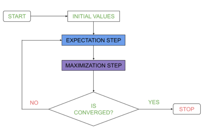
So, we had an understanding of the EM algorithm functionality but for implementation of this algorithm in python we need to understand the model which uses this algorithm to form clusters. Let’s talk about the Gaussian Mixture model.

Gaussian Mixture Model

The Gaussian Mixture Model is an important concept in machine learning which uses the concept of expectation-maximization. A Gaussian Mixture is composed of several Gaussians, each represented by ‘k’ which is the subset of the number of clusters to be formed. For each Gaussian ‘k’ in the mixture the following parameters are present:

• A mean of the data that defines the centre of the cluster.
• The covariance defines the cluster width. 
• The mixing probability of the Gaussian function determines the size of the function (big or small).

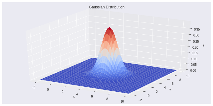
The above plot explains the Gaussian distribution for the data having a mean of 4 and a variance of 0.25. This could be concluded as the normal distribution. Using an iterative process the model concludes the final number of the cluster with the help of these parameters which determines the cluster stability.

How does GMM use Expectation-Maximization?

Let’s implement the concept of expectation-maximization in python.

Import necessary libraries

import numpy as np
import pandas as pd
import matplotlib.pyplot as plt
import plotly.express as px
import seaborn as sns
from sklearn.mixture import GaussianMixture
import warnings
warnings.filterwarnings('ignore')

Reading and analyzing the data

Using the famous wine data for this implementation.

df=pd.read_csv("/content/drive/MyDrive/Datasets/winequality-red.csv")
df.head()

Plotting a distribution

fig = px.histogram(df, x="residual sugar", y="total sulfur dioxide", color="quality",marginal='box',
                   hover_data=df.columns)
fig.show()

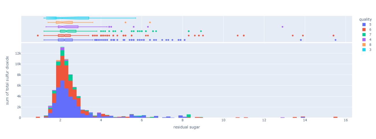
This plot helps to understand the distribution of the dependent variable over the independent variable.

Fitting the GMM

X=df.drop(['quality'],axis=1)
y=df['quality']
model = GaussianMixture(n_components=6, init_params='kmeans')
model.fit(X)
y_pred=model.predict(X)
model.score(X)

-0.7380311409986876

The score function returns the log-likelihood which the lower the better. The is negative because it is the product of the density evaluated at the observations and the density takes values that are smaller than one, so its logarithm will be negative. Ignoring the negative and focusing on the magnitude which is 0.73 indicates the model is good and the number of clusters should be 6.

Final Verdict

The expectation-Maximization Algorithm represents the idea of computing the latent variables by taking the parameters as fixed and known. The algorithm is inherently fast because it doesn’t depend on computing gradients. With a hands-on implementation of this concept in this article, we could understand the expectation-maximization algorithm in machine learning.

References

• Documentation of GMM
• Read what the wiki says about the EM algorithm
• Link to the above code