To maintain the reliability of the machine learning models, we need to improve their explainability and interpretability. There should be a proper reason that we can give while the model is making the predictions. Various tools help us in making the modelling procedure more explainable and interpretable. LIME is also a similar tool or package that gives the reason behind the predictions based on the data. In this article, we are going to discuss the LIME package and how we can implement it in our projects. We will learn how to explain the feature importance in machine learning with the help of this article. The major points to be discussed in the article are listed below.

Table of contents

1. What is LIME?
2. Implementation with lime
   1. Data preparation
   2. Model fitting
   3. Model interpretation
   4. Feature explanation

Let’s start with understanding what LIME is.

What is LIME?

LIME is an open-source package that enables us to explain the nature of models using visualization. The word LIME stands for Local Interpretable Model-agnostic explanations which means this package explains the model-based local values. This package is capable of supporting the tabular models, NLP models, and image classifiers. Using this package we can easily explain the answer of why the model is predicting a value.

The way this package follows to explain the results from the model is it tells about which features are responsible for making a result. It tells us about the strength of the result, what features are important in deriving results, and what values have been given to the model to predict the result. We can install this package in our environment using the following lines of codes.

!pip install lime

After the installation of Lime in the environment we are ready to use this package to make our models more interpretable. Let’s start with the implementation.     

Are you looking for for a complete repository of Python libraries used in data science, check out here.

Implementation of lime

In this article, we are going to use the multilayer perceptron model from the sklearn library and iris data that can be found here. Let’s just start by importing some important libraries and data.

Data preparation 

import numpy as np 
import pandas as pd
import seaborn as sns
from sklearn.model_selection import train_test_split
from sklearn import metrics

Let’s import the data 

data = pd.read_csv('/content/Iris.csv')
data.head()

Output:

Here we can see some of the values from our dataset. Let’s just visualize the data to understand the insights of the data. First, we will plot correlation:

corr = data.corr()
sns.heatmap(corr, 
xticklabels=corr.columns.values,
yticklabels=corr.columns.values)

Output:

In the above output, we can see the correlation between the features of the data. Let’s obtain a pair plot:

sns.pairplot( data=data, vars=('SepalLengthCm','SepalWidthCm','PetalLengthCm','PetalWidthCm'), hue='Species' )

Output: 

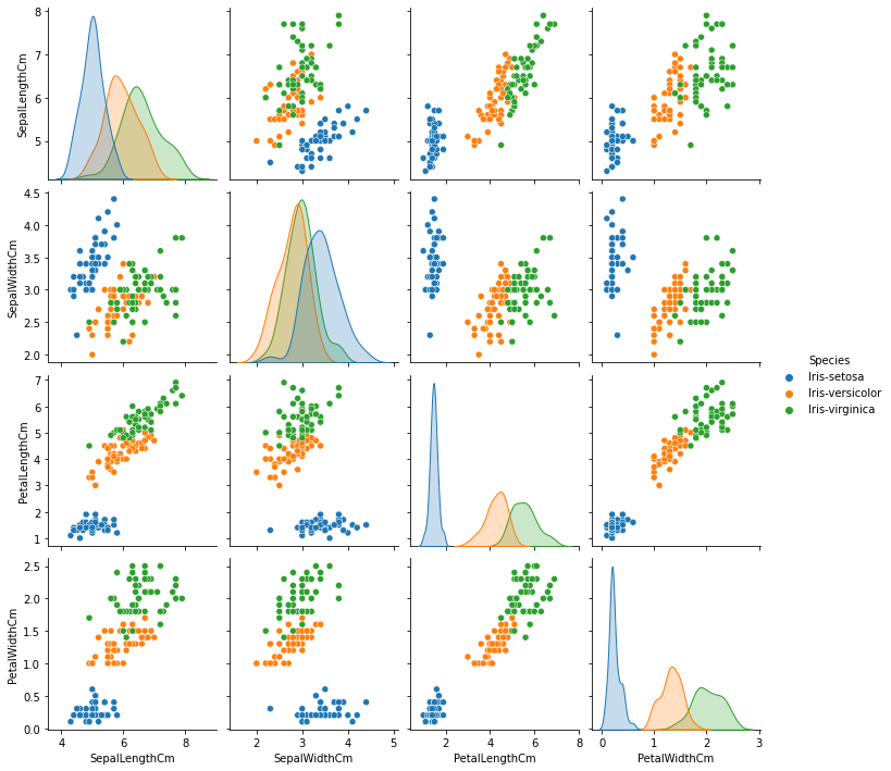
Here we can see the relations between the features more clearly. Let’s normalize the data:

df_norm = data[['SepalLengthCm', 'SepalWidthCm', 'PetalLengthCm', 'PetalWidthCm']].apply(lambda x: (x - x.min()) / (x.max() - x.min()))
df_norm.sample(n=5)

Output:

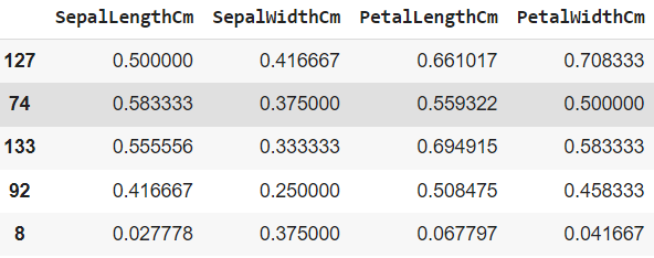
In the above, we have separated the target data from the features. For modelling the data we are required to provide numerical labels to the classes presented in the target variable.

target = data[['Species']].replace(['Iris-setosa','Iris-versicolor','Iris-virginica'],[0,1,2])
target.sample(5)

Output:

After normalizing and labelling the target and features let’s concatenate them again.

df = pd.concat([df_norm, target], axis=1)

Let’s split the data 

train, test = train_test_split(df, test_size = 0.3)
trainX = train[['SepalLengthCm','SepalWidthCm','PetalLengthCm','PetalWidthCm']]
trainY=train.Species
testX= test[['SepalLengthCm','SepalWidthCm','PetalLengthCm','PetalWidthCm']] 
testY =test.Species

After all the preparation we are ready to model the data using a multilayer perceptron classifier. Let’s define the model.

Model fitting 

from sklearn.neural_network import MLPClassifier
clf = MLPClassifier(solver='lbfgs', alpha=1e-5, hidden_layer_sizes=(3, 3), random_state=1)

Fitting the model with training data

clf.fit(trainX, trainY)

Output:

After fighting the model we are ready to check the accuracy of the model.

print('The accuracy of the Multi-layer Perceptron is:',metrics.accuracy_score(prediction,testY))

Output:

Let’s take a look at what are the predictions from model

print(prediction)

Output:

Here we have completed our modelling procedure and now we are ready to make this procedure interpretable using the LIME library.

Model interpretation 

Since we are using tabular data here, we are required to define a tabular explainer object using the lime library. This object will expect to provide values in the following parameters:

• Training_data: It simply asks for the data using which we have trained the model in the NumPy array format.
• feature_names: Name of the columns that have been provided to the model while training.
• class_name: Name of the classes in the target variable if we are building a classification model/
• mode:  The type of model we are building, here we have to build an MLP model for classification.

Let’s define the object.

import lime
from lime import lime_tabular
 
explainer = lime_tabular.LimeTabularExplainer(
    training_data=np.array(trainX),
    feature_names=trainX.columns,
    class_names=['Iris-setosa','Iris-versicolor','Iris-virginica'],
    mode='classification'
)

let’s make the explainer interpret the model based on the values available in the test set.

exp = explainer.explain_instance(
    data_row=testX.iloc[1], 
    predict_fn=clf.predict_proba
)
 
exp.show_in_notebook(show_table=True)

Output:

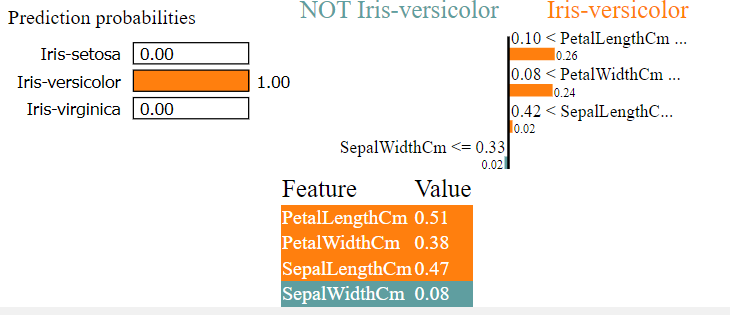
Here in the above, we have told the explainer to explain the prediction of the model on the second row of the test data. And we can see that the model is explaining the prediction is Iris_versicolor and in the middle, we can see that the graph is telling the reason why this sample is iris_versicolor. At the end we have a table that is telling about the value in test data and also telling that values in orange are the reason for the final prediction and values in the blue is not supporting the result.

Let’s check for any other row from the text data.

exp = explainer.explain_instance(
    data_row=testX.iloc[5], 
    predict_fn=clf.predict_proba
)
 
exp.show_in_notebook(show_table=True)

Output:

In the above, we can see that the explainer is telling that there is a 100% probability of the sample being Iris_virginica and what are the reasons for not being the Iris_versicolor.

Final words

In the article, we have discussed what LIME is and we have looked at an implementation using the iris data and MLPclassifier. At the final stages, we have discussed what and why the model is predicting anything using the tabular explainer of the LIME.

References

• Link for the codes
• Documentations of LIME