

Intent Classification, or you may say Intent Recognition is the labour of getting a spoken or written text and then classifying it based on what the user wants to achieve. This is a form of Natural Language Processing(NLP) task, which is further a subdomain of Artificial Intelligence. This technique finds vital application in chatbots (we all have seen and conversed with numerous chatbots on different websites). Use cases involve customer support, sales, gathering insights from Anonymous Chat Data (ACD), etc.
NLP, as defined, is concerned with computation and processing, analyzing and extracting features out of natural language. One may think how it is different from Text Classification and Question Answering; the answer is given below in the following example for better understanding.
Let’s take two sentences from a chat; these are-
- I am hungry.
- I have not eaten anything since morning.
These two sentences have different syntactic meanings – these are seen as facts when solving classical Text Classification problems. But let’s try and take a look from some other view (intent of the sentences). Sentence 1 sure shot says that the person is hungry. Sentence 2, however, does not contain the word hungry, yet we can understand the ‘intent’ of the person he or she is hungry at that moment considering not eating anything.
Recognizing intents like this and so many others is the task we have to achieve. This can be done using BERT (a simple stack of encoders on top of one another) as we have to understand what the sentence is telling us. Annotated data, that is the data should be labelled with intent; hence it is a supervised problem statement.
The rise of chatbots is in the direction of user trust in chatbots, gaining more popularity. A survey by Helpshift found out that the number of people willing to use chatbots was twice in 2019 as that of 2018. This is because of obvious reasons with the advancements in text models and in time support. Not only it saves unimaginable human hours but it gives humongous profits.
This article will use a pre-trained BERT model that will be huge (leveraging the model checkpoints) and fine-tune it to our needs with labelled text data with seven intents. The data is divided into three parts, namely – train test and validity. All the data will be provided for you to download in the form of a zip file here. This contains the model architecture as well as the datasets we are going to use. The datasets are pre-processed to make this article sufficiently enough; else we’ll be at it for hours. Saving all that time, we’ll write up some functions for encoding and then define the model accordingly.
Let’s jump into the coding part already.
Code Implementation of Intent Recognition with BERT
Importing Necessary Dependencies
 # checking for the GPU we get for this model
 !nvidia-smi
 # installing the latest version of tensorflow GPU
 !pip install tensorflow-gpu >> /dev/null
 !pip install --upgrade grpcio >> /dev/null
 # show progress bars while installation and downloading
 !pip install tqdm  >> /dev/null
 # the original implementation given in research paper is not compatible with TensorFlow 2. The bert-for-tf2 package solves this issue.
 !pip install bert-for-tf2 >> /dev/null
 # install sentencepiece tokenizer for making tokens out of sentences
 !pip install sentencepiece >> /dev/null
 # making directories, math operations
 import os
 import math
 import datetime
 # show progress bars in the notebook itself
 from tqdm import tqdm
 # data manipulation in dataframe and array
 import pandas as pd
 import numpy as np
 # keras implementation
 import tensorflow as tf
 from tensorflow import keras
 # import the bert model and model layer
 # also the bert tokenizer for text pre processing
 import bert
 # we can change the layers downloaded from here
 from bert import BertModelLayer
 # useful for loading necessary files from data
 from bert.loader import StockBertConfig, map_stock_config_to_params, load_stock_weights
 from bert.tokenization.bert_tokenization import FullTokenizer
 # data visualization at the time of data import and model metrics
 import seaborn as sns
 # we can set the parameters for each plot
 from pylab import rcParams
 import matplotlib.pyplot as plt
 from matplotlib.ticker import MaxNLocator
 from matplotlib import rc
 # model metrics to be defined
 from sklearn.metrics import confusion_matrix, classification_report
 # showing the plots in the notebook itself
 %matplotlib inline
 # retina is a style shape
 %config InlineBackend.figure_format='retina'
 # setting the visualizing settings first hand
 sns.set(style='whitegrid', palette='muted', font_scale=1.2)
 # getting the colors we need for plots
 HAPPY_COLORS_PALETTE = ["#01BEFE", "#FFDD00", "#FF7D00", "#FF006D", "#ADFF02", "#8F00FF"]
 # define the color palette
 sns.set_palette(sns.color_palette(HAPPY_COLORS_PALETTE))
 # size can be set accordingly
 rcParams['figure.figsize'] = 12, 8
 # generating pseudo random numbers
 RANDOM_SEED = 42
 # np arrays , tensors
 np.random.seed(RANDOM_SEED)
 tf.random.set_seed(RANDOM_SEED)
Downloading Data and Model zip
 # downloading the data from google drives which is in now form of csv files having two columns of sentences and it's intent
 # earlier the data was in form of json file but after a little bit of data pre processing , we are using it in the form of csv files
 !gdown --id 1OlcvGWReJMuyYQuOZm149vHWwPtlboR6 --output train.csv
 !gdown --id 1Oi5cRlTybuIF2Fl5Bfsr-KkqrXrdt77w --output valid.csv
 !gdown --id 1ep9H6-HvhB4utJRLVcLzieWNUSG3P_uF --output test.csv
 # making separate dataframes for the three files
 # which are already pre processed
 train = pd.read_csv("train.csv")
 valid = pd.read_csv("valid.csv")
 test = pd.read_csv("test.csv")
 # appending the valid df to train df to make a bigger data
 train = train.append(valid).reset_index(drop=True)
 # training df has 13784 no. of records
 # 13,784 data points with intents
 train.shape
 train.head()
 # let's check how the datset looks , if it is imbalanced or not
 # making a chart to see how many texts are for each of the seven intents
 chart = sns.countplot(train.intent, palette=HAPPY_COLORS_PALETTE)
 # setting title of the chart
 plt.title("Number of texts per intent")
 # setting labels to the bottom at an angle of 30 degrees
 chart.set_xticklabels(chart.get_xticklabels(), rotation=30, horizontalalignment='right');
While running the code, after running this, we see that the dataset is balanced.
 # download the pre trained bert model in the form of a zip file
 !wget https://storage.googleapis.com/bert_models/2018_10_18/uncased_L-12_H-768_A-12.zip
 # unzipping the file having model
 # this is having all the checkpoints , vocab.text for tokenizer , configurations for model
 !unzip uncased_L-12_H-768_A-12.zip
 # make a folder named model for moving all the stuff
 os.makedirs("model", exist_ok=True)
 # moving the stuff from bert to model folder
 !mv uncased_L-12_H-768_A-12/ model
 # specify the model name
 bert_model_name="uncased_L-12_H-768_A-12"
 # specify where the  check point directory is
 bert_ckpt_dir = os.path.join("model/", bert_model_name)
 # specify the checkpoint file itself
 bert_ckpt_file = os.path.join(bert_ckpt_dir, "bert_model.ckpt")
 # specify the configuration file
 bert_config_file = os.path.join(bert_ckpt_dir, "bert_config.json")
PreProcessing
 # pre processing in which we have to use the tokenizer
 # for getting tokens so that we can feed the model
 # creating a class which is a little generic for doing our tokenizing process
 class IntentDetectionData:
   # we had two columns to which have given names according to use
   DATA_COLUMN = "text"
   LABEL_COLUMN = "intent"
   '''
   creating constructor having train data , test data , tokenzier , max_seq_len because NLP tasks work on a fixed number of elements
   the data set we are having has different lengths of sequences , that's why we have to do same length for all  , either we can cut the sequence
   lengths to some minimal point or we can add padding up to the maximum existing
   '''
   def __init__(self, train, test, tokenizer: FullTokenizer, classes, max_seq_len=192):
     self.tokenizer = tokenizer
     # setting initial to 0
     self.max_seq_len = 0
     self.classes = classes
     '''
     create train_X and train_Y
     train_X will have the vectors , train_Y will have the target labels
     same we will do for the testing part
     '''
     train, test = map(lambda df: df.reindex(df[IntentDetectionData.DATA_COLUMN].str.len().sort_values().index), [train, test])
     # we gave to set the variables to which we can map values using the above function
     ((self.train_x, self.train_y), (self.test_x, self.test_y)) = map(self._prepare, [train, test])
     print("max seq_len", self.max_seq_len)
     # setting the actual value to max_seq_len
     self.max_seq_len = min(self.max_seq_len, max_seq_len)
     # adding padding in the following line
     self.train_x, self.test_x = map(self._pad, [self.train_x, self.test_x])
   def _prepare(self, df):
     # initialising two empty arrays
     x, y = [], []
     # iterate over each row and use tqdm to visualize that
     for _, row in tqdm(df.iterrows()):
       # extracting the seq. and labels
       text, label = row[IntentDetectionData.DATA_COLUMN], row[IntentDetectionData.LABEL_COLUMN]
       # create an object named token and initialise it
       tokens = self.tokenizer.tokenize(text)
       # adding two special tokens which will surround each token
       # from front and back
       tokens = ["[CLS]"] + tokens + ["[SEP]"]
       # convert the token ids to numbers using a helper
       # function already provided for feeding
       token_ids = self.tokenizer.convert_tokens_to_ids(tokens)
       # calculate the length of seq. by taking max.
       self.max_seq_len = max(self.max_seq_len, len(token_ids))
       # appends the token ids to x
       x.append(token_ids)
       # indexes of labels to the y
       y.append(self.classes.index(label))
     # returning these in the form of nparrays
     return np.array(x), np.array(y)
   # takes the ids and not the tokens itself
   def _pad(self, ids):
     # create an empty list again
     x = []
     # iterating over each id
     for input_ids in ids:
       # we have to cut the longer seq. , self.max_seq_len - 2
       # because two positions are reserved for the special tokens as mentioned before
       input_ids = input_ids[:min(len(input_ids), self.max_seq_len - 2)]
       # adding padding to the smaller ones
       input_ids = input_ids + [0] * (self.max_seq_len - len(input_ids))
       # appending
       x.append(np.array(input_ids))
     return np.array(x)
 # use tokenizer which expects a vocabulary file,
 # we have this file already in our data
 tokenizer = FullTokenizer(vocab_file=os.path.join(bert_ckpt_dir, "vocab.txt"))
 # trying the tokenizer , lower cases everything , good tokenizer as it preserves punctuations
 tokenizer.tokenize("I can't wait to visit India again!")
 # example of tokenization and then converting them to token ids which are basically numbers for our model to understand
 tokens = tokenizer.tokenize("I can't wait to visit India again!")
 tokenizer.convert_tokens_to_ids(tokens)
Model
 # create model to use the pre trained bert model and convert it into intent recogniser by adding keras layers
 # parameters are to be the max_seq_len , checkpoint file
 def create_model(max_seq_len, bert_ckpt_file, bert_config_file):
   # open the config file using tensorflow for reading
   with tf.io.gfile.GFile(bert_config_file, "r") as reader:
     # using this variable read the config file
       bc = StockBertConfig.from_json_string(reader.read())
       bert_params = map_stock_config_to_params(bc)
       # adapter_size is for fine tune the model faster
       bert_params.adapter_size = None
       # this is the bert model named simply bert for ease
       # this is actually very huge stack of keras layers
       bert = BertModelLayer.from_params(bert_params, name="bert")
   # create the input layer with seq. len as input
   input_ids = keras.layers.Input(shape=(max_seq_len, ), dtype='int32', name="input_ids")
   # output from the bert model is being saved here
   # to which we provided our processed data (ids)
   bert_output = bert(input_ids)
   # printing the shape of bert model
   print("bert shape", bert_output.shape)
   # use lambda layer from keras , taking the first layer out of those 38 layers
   # and rest we have taken all 768
   cls_out = keras.layers.Lambda(lambda seq: seq[:, 0, :])(bert_output)
   # drop out layers to prevent overfitting using the keras API with 50% probability
   cls_out = keras.layers.Dropout(0.5)(cls_out)
   # flatten this using the dense layer , activation function used hai tanh
   logits = keras.layers.Dense(units=768, activation="tanh")(cls_out)
   # adding one more drop out layer
   logits = keras.layers.Dropout(0.5)(logits)
   # dense o/p layer , activation to be used is softmax as this is classification
   logits = keras.layers.Dense(units=len(classes), activation="softmax")(logits)
   # this is going to be a keras model , i/p - input_ids , o/p - logits from the last layer
   model = keras.Model(inputs=input_ids, outputs=logits)
   '''
   building the model and specify the i/p shape of this whole model
   the first parameter is None because this will be initialised by keras for us
   '''
   model.build(input_shape=(None, max_seq_len))
   # load the weights
   load_stock_weights(bert, bert_ckpt_file)
   return model
 # taking unique intents and convert them to list
 classes = train.intent.unique().tolist()
 # already defined function which we created earlier
 data = IntentDetectionData(train, test, tokenizer, classes, max_seq_len=128)
 # we can see the test and train data by running this cell
 # these many token ids with these many seq. len
 data.train_x.shape
 # this is how a data point looks
 data.train_x[0]
 # this is a single id
 data.train_y[0]
 # max len of token ids
 data.max_seq_len
 # create the model with three input parameters
 model = create_model(data.max_seq_len, bert_ckpt_file, bert_config_file)
 # we get some unused weights
 '''
 these are the layers that we put earlier in our model
 bert layer has around 108 mil param
 last dense layer will have the o/p only which is 7 classes
 '''
 model.summary()

 # compiling the model
 model.compile(
   # optimizer is Adam with learning rate 0.00001 ,  this is recommended by authors of bert model paper
   optimizer=keras.optimizers.Adam(1e-5),
   # using SparseCategoricalCrossentropy
   # because we have not used OneHotencoding here
   loss=keras.losses.SparseCategoricalCrossentropy(from_logits=True),
   # specify the metrics from keras
   metrics=[keras.metrics.SparseCategoricalAccuracy(name="acc")]
 )
 # use a tensorboard callback so that we can see the training processafter everything is completed
 log_dir = "log/intent_detection/" + datetime.datetime.now().strftime("%Y%m%d-%H%M%s")
 # create a callback from keras
 tensorboard_callback = keras.callbacks.TensorBoard(log_dir=log_dir)
 # finally fit the model
 history = model.fit(
   x=data.train_x,
   y=data.train_y,
   # validation split to be 10% of the data
   validation_split=0.1,
   # recommendation from authors , batch to be 16
   batch_size=16,
   # yes we want to shuffle
   shuffle=True,
   # another recommendation from authors
   epochs=5,
   # specify the call back
   callbacks=[tensorboard_callback]
 )
 # showing the tensorboard
 %tensorboard --logdir log
Output
 # how loss has decreased with epoch number
 ax = plt.figure().gca()
 ax.xaxis.set_major_locator(MaxNLocator(integer=True))
 ax.plot(history.history['loss'])
 ax.plot(history.history['val_loss'])
 plt.ylabel('Loss')
 plt.xlabel('Epoch')
 plt.legend(['train', 'test'])
 plt.title('Loss over training epochs')
 plt.show();
 # graph for accuracy against the epoch number
 ax = plt.figure().gca()
 ax.xaxis.set_major_locator(MaxNLocator(integer=True))
 ax.plot(history.history['acc'])
 ax.plot(history.history['val_acc'])
 plt.ylabel('Accuracy')
 plt.xlabel('Epoch')
 plt.legend(['train', 'test'])
 plt.title('Accuracy over training epochs')
 plt.show();
 # evaluate the test accuracy , call evaluate method and give the data
 _, train_acc = model.evaluate(data.train_x, data.train_y)
 _, test_acc = model.evaluate(data.test_x, data.test_y)
 print("train acc", train_acc)
 print("test acc", test_acc)
 # take the class that is most likely to be the correct one based on model's opinion
 y_pred = model.predict(data.test_x).argmax(axis=-1)
Prediction with examples
 # print classification report
 print(classification_report(data.test_y, y_pred, target_names=classes))
 # create a confusion matrix and chart it
 cm = confusion_matrix(data.test_y, y_pred)
 df_cm = pd.DataFrame(cm, index=classes, columns=classes)
 # using a heatmap from seaborn to visualize the confusion matric
 hmap = sns.heatmap(df_cm, annot=True, fmt="d")
 hmap.yaxis.set_ticklabels(hmap.yaxis.get_ticklabels(), rotation=0, ha='right')
 hmap.xaxis.set_ticklabels(hmap.xaxis.get_ticklabels(), rotation=30, ha='right')
 plt.ylabel('True label')
 plt.xlabel('Predicted label');
 # trying a few sentences which the model has not seen
 sentences = [
   "HEAR MUSIC",
   "Rate this book as awful"
 ]
 pred_tokens = map(tokenizer.tokenize, sentences)
 pred_tokens = map(lambda tok: ["[CLS]"] + tok + ["[SEP]"], pred_tokens)
 pred_token_ids = list(map(tokenizer.convert_tokens_to_ids, pred_tokens))
 pred_token_ids = map(lambda tids: tids +[0]*(data.max_seq_len-len(tids)),pred_token_ids)
 pred_token_ids = np.array(list(pred_token_ids))
 predictions = model.predict(pred_token_ids).argmax(axis=-1)
 for text, label in zip(sentences, predictions):
   print("text:", text, "\nintent:", classes[label])
   print()
 model.save('Bert.h5')

EndNote
As we can see in the output, the model has successfully recognized the intent on never seen examples. I recommend the readers to try this model on different datasets, altering the model hyperparameters. This is a beautiful, more pythonic way of implementing a model so make sure to understand why generic functions in such a big model are vital.