|
Listen to this story
|
Time series analysis, is one of the major parts of data science and techniques like clustering, splitting and cross-validation require a different kind of understanding of the data. In one of our articles, we have discussed the clustering of time series. In this article, we are going to discuss cross-validation in time series. The major points to be discussed in the article are listed below.
Table of contents
- Simple cross-validation
- Cross-validation in time series
- k-fold Cross-Validation on Time Series
- Implementation of k-fold cross-validation
- Comparison between k-fold cross-validation and general modelling
- General modelling
- Modelling with cross-validation
Let’s briefly revise what is cross-validation?
simple cross-validation
In general, cross-validation is one of the methods to evaluate the performance of the model. It works by segregation data into different sets and after segregation, we train the model using these folds except for one fold and validate the model on the one fold. This type of validation requires to be performed many times.
The final result we form using the average of scores obtained in every fold. Using this type of modelling procedure we try to prevent the overfitting and check the accuracy of models while considering the robustness of the model. The below image represents the idea behind the cross-validation
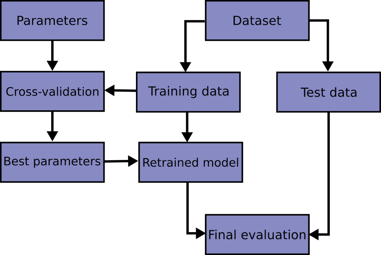
In the above, we can see the base concept behind the cross-validation and there are different techniques for performing cross-validation like k-fold, stratified k-fold, Rolling, and Holdout. Here we are going to discuss the cross-validation.
Are you looking for a complete repository of Python libraries used in data science, check out here.
Cross-validation in time series
We need to think about cross-validation in time series differently because it works on a rolling basis. In general, cross-validation can bethink as randomly picking some data from the whole data and we perform the next analysis on that picked up data. When these things come on the time series data we are required to know that the time series data generates when variables are changing with time. By this, we can understand the data point we get in the time series is closely correlated to previous data and we can not pick these kinds of data randomly.
One example of performing cross-validation on the data can be thought of as choosing the data based on time, not by the percentage. Step by step performing the analysis based on time can increase the efficiency of the model by understanding the sequence of the data.
k-fold Cross-Validation in Time Series
We need to think about cross-validation in time series differently because it works on a rolling basis. As we know the data that a time series includes is sequential and often correlated to its last data point. In such an environment, cross-validation is required to perform while the model is forecasting. Once the model starts forecasting, the accuracy of the forecasted points is checked and then some of the forecasted data points with older data are required for making the next predictions.
Let’s take an intuition from the below picture.
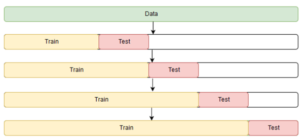
Image source
In the above image, we can see how cross-validation works with the time series data. The idea behind the cross-validation of time series can be more explainable while taking an example of simple data.
Let’s say [1, 2, 3, 4, 5] is our data. Here we are required to perform k-fold cross-validation and the value of k is 4.
According to the k-fold cross-validation, we are required to make 4 pairs of training and test data that can be done using g the following rules:
- There should be new observations in the test set
- The training set observations come first, followed by the test set observations.
Let’s take a look at the way to generate such pairs from the dataset.
- Train data: [1] Test data: [2]
- Train data: [1, 2] Test data: [3]
- Train data: [1, 2, 3] Test data: [4]
- Train data: [1, 2, 3, 4] Test data: [5]
- Compute the average of the accuracies of the 4 test folds.
Here we can see how the cross-validation works and we can understand that the cross-validation in time series is different from the general modelling.
Implementation of k-fold cross-validation
Let’s take a look at how we can perform this using python.
import numpy as np
from sklearn.model_selection import TimeSeriesSplit
X = np.array([[1, 2], [3, 4], [1, 2], [3, 4], [1, 2], [3, 4]])
y = np.array([1, 2, 3, 4, 5, 6])
cv = TimeSeriesSplit()
for train_index, test_index in tscv.split(X):
    print("Train data:", train_index, "Test data:", test_index)
    X_train, X_test = X[train_index], X[test_index]
    y_train, y_test = y[train_index], y[test_index]
0utput:

Here is an example of performing k-fold cross-validation with the time series data.
Comparison between k-fold cross-validation and general modelling
We can compare general modelling and modelling with cross-validation while implementing both the procedure. Let’s take a look at the procedure using which we can enhance the performance of time series modelling.
General modelling
Let’s first Import the data.
import pandas as pd
path = '/content/drive/MyDrive/Yugesh/deseasonalizing time series/AirPassengers.csv'
data = pd.read_csv(path, index_col='Month')
data.head(20)
output
path = ‘/content/drive/MyDrive/Yugesh/deseasonalizing time series/AirPassengers.csv’
data = pd.read_csv(path, index_col=’Month’)
data.head(20)
Output:
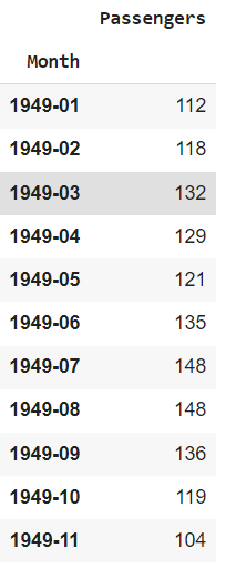
Here in this article, we are going to use the Airline data set that consists of the number of passengers an airline consists of in a month. This data can be downloaded from here. Let’s split the data into train and test.
#divide data into train and test
train_ind = int(len(data)*0.8)
train = data[:train_ind]
test = data[train_ind:]
Now after splitting we can fit and train a simple exponential model in the following ways.
from statsmodels.tsa.holtwinters import ExponentialSmoothing
from sklearn.metrics import mean_squared_error
from math import sqrt
model = ExponentialSmoothing(train, seasonal='mul', seasonal_periods=12).fit()
pred = model.predict(start=test.index[0], end=test.index[-1])
MSE=round(mean_squared_error(test, pred),2)
MSE
from statsmodels.tsa.holtwinters import ExponentialSmoothing
from sklearn.metrics import mean_squared_error
from math import sqrt
model = ExponentialSmoothing(train, seasonal=’mul’, seasonal_periods=12).fit()
pred = model.predict(start=test.index[0], end=test.index[-1])
MSE=round(mean_squared_error(test, pred),2)
MSE
Output:

Here, we can see the MSE between the test and predictions from the model. Now let’s perform this similar modelling with a cross-validation procedure.
Modelling with cross-validation
In the above sections, we have looked at how the k-fold cross-validation works with the time series. Here we don’t need to split our data set because the defined numbers of k will make a fold of the data and train the model on them. Let’s start with performing k-fold on the data.
from sklearn.model_selection import TimeSeriesSplit
tscv = TimeSeriesSplit(n_splits=5)
for train_index, test_index in tscv.split(data):
  print('TRAIN:', train_index, 'TEST:', test_index)
  X_train, X_test = data.Passengers[train_index], data.Passengers[test_index]
  y_train, y_test = data.index[train_index], data.index[test_index]
Output:
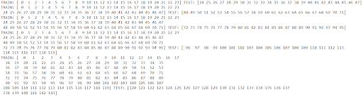
Here in the above, we can see that our folds are prepared. Now let’s segregate our data based on the above folds.
#Splitting according to the above description
train1, test1 = data.iloc[:24, 0], data.iloc[24:48, 0]
train2, test2 = data.iloc[:48, 0], data.iloc[48:72, 0]
train3, test3 = data.iloc[:72, 0], data.iloc[72:96, 0]
train4, test4 = data.iloc[:96, 0], data.iloc[96:120, 0]
train5, test5 = data.iloc[:120, 0], data.iloc[120:144, 0]
After the split, we are required to fit the models in the folds.
model1 = ExponentialSmoothing(train1, seasonal='mul', seasonal_periods=12).fit()
pred1 = model1.predict(start=test1.index[0], end=test1.index[-1])
MSE1=round(mean_squared_error(test1, pred1),2)
model2 = ExponentialSmoothing(train2, seasonal='mul', seasonal_periods=12).fit()
pred2 = model2.predict(start=test2.index[0], end=test2.index[-1])
MSE2=round(mean_squared_error(test2, pred2),2)
model3 = ExponentialSmoothing(train3, seasonal='mul', seasonal_periods=12).fit()
pred3 = model3.predict(start=test3.index[0], end=test3.index[-1])
MSE3=round(mean_squared_error(test3, pred3),2)
model4 = ExponentialSmoothing(train4, seasonal='mul', seasonal_periods=12).fit()
pred4 = model4.predict(start=test4.index[0], end=test4.index[-1])
MSE4=round(mean_squared_error(test4, pred4),2)
model5 = ExponentialSmoothing(train5, seasonal='mul', seasonal_periods=12).fit()
pred5 = model5.predict(start=test5.index[0], end=test5.index[-1])
MSE5=round(mean_squared_error(test5, pred5),2)
After fitting these models let’s check all MSE values between the test data and prediction
model1 = ExponentialSmoothing(train1, seasonal=’mul’, seasonal_periods=12).fit()
pred1 = model1.predict(start=test1.index[0], end=test1.index[-1])
MSE1=round(mean_squared_error(test1, pred1),2)
model2 = ExponentialSmoothing(train2, seasonal=’mul’, seasonal_periods=12).fit()
pred2 = model2.predict(start=test2.index[0], end=test2.index[-1])
MSE2=round(mean_squared_error(test2, pred2),2)
model3 = ExponentialSmoothing(train3, seasonal=’mul’, seasonal_periods=12).fit()
pred3 = model3.predict(start=test3.index[0], end=test3.index[-1])
MSE3=round(mean_squared_error(test3, pred3),2)
model4 = ExponentialSmoothing(train4, seasonal=’mul’, seasonal_periods=12).fit()
pred4 = model4.predict(start=test4.index[0], end=test4.index[-1])
MSE4=round(mean_squared_error(test4, pred4),2)
model5 = ExponentialSmoothing(train5, seasonal=’mul’, seasonal_periods=12).fit()
pred5 = model5.predict(start=test5.index[0], end=test5.index[-1])
MSE5=round(mean_squared_error(test5, pred5),2)
After fitting these models let’s check all MSE values between the test data and prediction
print ("MSE:", MSE)
print ("MSE1:", MSE1)
print ("MSE2:", MSE2)
print ("MSE3:", MSE3)
print ("MSE4:", MSE4)
print ("MSE5:", MSE5)
print (“MSE1:”, MSE1)
print (“MSE2:”, MSE2)
print (“MSE3:”, MSE3)
print (“MSE4:”, MSE4)
print (“MSE5:”, MSE5)
Output:
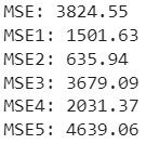
Here we can see that some of the folds have performed very well because their MSE value is lower than the general model.
Now let’s check for the overall MSE value.
Overall_MSE=round((MSE1+MSE2+MSE3+MSE4+MSE5)/5,2)
print ("Overall MSE:", Overall_MSE)
Output:

Here we can see that our overall MSE while performing k-fold cross-validation is much better than the general modelling. This is how we can improve the performance of the time series modelling.
Final words
In this article, we have discussed the cross-validation in time series that needs to perform differently because in the time series the data points we have correlates with the lagged values. Along with this, we have discussed how we can do it using the sklearn package and a comparison between the general modelling and modelling with cross-validation.