Testing a predictive model plays a crucial role in machine learning. We usually evaluate these models by optimizing some loss functions with respect to the parameters defined by the model. In-depth, we can optimize these loss functions using gradient descent. Autograd is a python package that can help us in optimizing various functions whether they are related to machine learning models or related to core mathematics. This package can also replace the popular NumPy library in various cases. In this article, we will discuss the Autograd package and we will understand how we can use it. The major points to be discussed in this article are listed below. 

Table of contents

1. What is Autograd?
2. Implementation of Autograd
   1. Evaluating the gradient of the hyperbolic tangent function
   2. Optimizing loss functions in Logistic regression     

Let us start with having an introduction with Autograd.

What is Autograd?

Autograd is a python package that can provide us with a way to differentiate Numpy and Python code. It is a library for gradient-based optimization. Using this package we can work with a large subset of features of python including loops, ifs, recursion, and closures. Also, this package is capable of taking multiple step-wise derivatives of functions. Most of the time we find that this package supports the backpropagation and forward propagation methods that can also be called reverse-mode differentiation and forward mode differentiation in mathematics, which means this package is capable of picking gradients from a function with scalar values.  

Using this package we can compose these two methods arbitrarily. Basically, this package is intended to provide us with the facility of gradient-based optimization. Using this package we can utilize gradients for the following operations and functions:

• Mathematical operations – various gradients are implemented for optimizing most of the mathematical operations.
• Gradients for completing various array manipulation are available.
• Gradients for completing various matrix manipulations are in the package.
• Various gradients are in the package for some linear algebra and Fourier transform routines.
• Modules are there for N-dimensional convolutions.
• Full support for complex numbers.

We can install this package using the following lines of codes:

!pip install autograd

After installing this package in the environment, we are ready to use this package for our work.        

Are you looking for for a complete repository of Python libraries used in data science, check out here.

Implementations of Autograd

In this section of the article, we will look at some of the functions that can be followed using the Autograd package.

Evaluating the gradient of the hyperbolic tangent function 

In this implementation, we will look at how we can evaluate the gradient of the Tanh function. Let’s define the function.

import autograd.numpy as agnp
def tanh(x):                 
     y = agnp.exp(-2.0 * x)
     return (1.0 - y) / (1.0 + y)

In the above codes, we can see that we have used module autograd.numpy which is a wrapper of NumPy in the autograd package. Also, we have defined a function for tan. Let’s evaluate the gradient of the above-defined function.

from autograd import grad 
grad_tanh = grad(tanh)    
grad_tanh(1.0)

Output: 

Here in the above codes, we have initiated a variable that can hold the tanh function and for evaluation, we have imported a function called grad from the autograd package. Let’s compare the finite range difference.

(tanh(1.0001) - tanh(0.9998)) / 0.0002 

Output:

We also have the facility to differentiate the functions as many times as we want, for this, we just need to call a module named as the elementwise_grad.

from autograd import elementwise_grad
x = agnp.linspace(-10, 10, 100)

In the above codes, we have called our module and defined an array having random values between -10 to 10. In this, we will try to draw derivatives for the above-defined function.

plt.plot(x, agnp.tanh(x),
         x, elementwise_grad(agnp.tanh)(x),
         x, elementwise_grad(elementwise_grad(agnp.tanh))(x),
         x, elementwise_grad(elementwise_grad(elementwise_grad(agnp.tanh)))(x),
         x, elementwise_grad(elementwise_grad(elementwise_grad(elementwise_grad(agnp.tanh))))(x))        
plt.show()

Output:

Here we can see how the function is varying for our defined x.

Note- at the very start of the implementation we have defined a function of tanh and here in the recent one we have used the function given by autograd.    

In the above example, we have discussed how to use modules from autograd. Let’s see how we can use it for logistic regression.

Optimizing loss functions in Logistic regression 

Let’s define a sigmoid function.

def function1(x):
    return 0.5 * (agnp.tanh(x / 2.) + 1)

Defining a function for predictions:

def function2(w, i):
    return function1(agnp.dot(i, w))

Defining loss function for training:

def loss_function(w):
    preds = function2(w, i)
    label_probabilities = preds * targets + (1 - preds) * (1 - targets)
    return -agnp.sum(agnp.log(label_probabilities))

Defining the weights  and input:

i = agnp.array([[0.52, 1.12,  0.77],                
                [0.88, -1.08, 0.15],
                [0.52, 0.06, -1.30],
                [0.74, -2.49, 1.39]])
w = agnp.array([0.0, 0.0, 0.0])

Defining the target:

targets = agnp.array([True, True, False, True])

Defining gradient function for training loss:

training_gradient = grad(loss_function)

Optimization of weight using the gradient descent:

w = np.array([0.0, 0.0, 0.0])
print("loss in initial:", loss_function(w))
for i in range(100):
    weights -= training_gradient(w) * 0.01
print("loss after training:", loss_function(w))

Output:

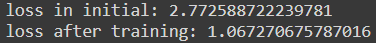
Here we have seen an example of logistic regression for optimization of weights that we pushed in between using the modules of the autograd package. 

Final words

In this article, we have discussed what Autograd is, which is a package for gradient-based optimization of various functions. Along with this, we have gone through some of the implementations for optimizing functions related to mathematics and machine learning.    

References

• Link for the above codes 
• Documentation of autograd