

Learning rate is an important parameter in neural networks for that we often spend much time tuning it and we even don’t get the optimum result even trying for some different rates. The learning rate annealing comes to the picture here, in which we have certain methods to traverse around different learning in various fashions to get optimal cost function. In this post, we are going to discuss what learning rate annealing and at the last, we practically see the difference between the standard and annealing process in neural networks. The major points to be discussed are listed below.
Table of Contents
- Learning Rate
- What is Learning Rate Annealing?
- Methods of Learning Rate Annealing
- Implementing Learning Annealing in Python
Let’s start the discussion by understanding the paradigm of learning rate.
Learning Rate
One of the first and most significant aspects of a model is the learning rate, which you should start thinking about almost soon after starting to develop one. It determines the size of the jumps your model makes and, as a result, how rapidly it learns.
Neural networks learn by applying gradient descent to your data across a network of nodes, resulting in a set of nodal weights that are predictive of the values in your target when combined. The goal of the gradient descent process we employ to learn with our neural network can be thought of as the algorithm which tries to find the optimum solution for a given instance by traversing over all the points and trying to model the data. The rate at which it traverses is defined as the learning rate.
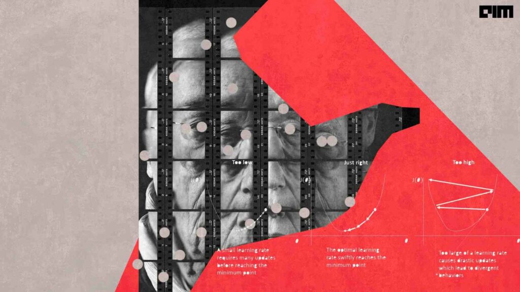
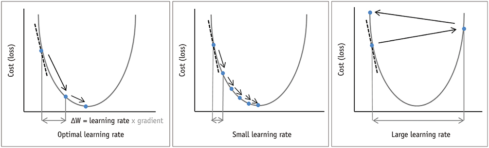
Your neural network will take a long time to converge if you set a learning rate that is too low. If you choose an excessively high learning rate, you will be presented with a new and more fascinating challenge. For most purposes, think of gradient descent as moving around on an uneven, very lumpy, and perhaps non-convex cost surface like the one shown in the image above.
The appropriate learning rate is determined by the topology of your loss landscape, which is determined by your model architecture and dataset. While the default learning rate may yield satisfactory results, finding an optimal learning rate can often increase performance or speed up training that’s where term learning rate annealing came into the picture.
What is Learning Rate Annealing?
Changing the learning rate for your stochastic gradient descent optimization technique can improve performance while also cutting down on training time. This is also known as adaptable learning rates or learning rate annealing. This method is referred to as a learning rate schedule since the default schedule updates network weights at a constant rate for each training period.
Techniques that reduce the learning rate over time are the simplest and arguably most commonly used modification of the learning rate during training. These have the advantage of making big modifications at the start of the training procedure when larger learning rate values are employed and decreasing the learning rate later in the training procedure when a smaller rate and hence smaller training updates are made to weights.
Methods of Learning Rate Annealing
A Learning Rate Decay
The way things will evolve throughout time is defined by a schedule. The learning rate schedule, in general, defines a learning rate for each epoch and batch. For scheduling global learning rates, there are two sorts of methods: decay and cyclical. The learning rate annealing approach, which is scheduled to progressively decay the learning rate during the training process, is the most popular method.
In order to get a stronger generalization effect, a somewhat big step size is preferred in the early stages of training. The stochastic noise is reduced when the learning rate decreases. This helps the algorithm converge by avoiding oscillation at the ideal spot.

The step (staircase) decay and the exponential decay are two popular learning rate decay approaches. In practice, the staircase method reduces the learning rate in multiple step intervals and produces a nice effect. The exponential decay slows down the learning rate for each step, resulting in a smooth curve. The learning rate schedules of the staircase type are depicted in the diagram above.
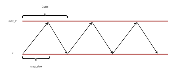
The cyclical method (shown above), on the other hand, involves repeating a learning rate period with an upper and lower bound over epochs. The cyclic technique is based on the observation that raising the learning rate in the optimization process can have a detrimental impact, but it can also result in better generalization of the trained model. A single decay, such as the exponential decay and step decay methods, or a triangle function can be used for the learning rate period.
Adaptive Learning Rate
It is desirable to automatically calculate the step size in gradient-based optimization based on the loss gradient that indicates the convergence of each of the unknown parameters. To this end, parameter-wise adaptive learning rate scheduling algorithms have been developed, such as AdaGrad, AdaDelta, RMSprop, and Adam, which allow the process to quickly converge in practice. The adaptive technique has recently been used to combine Adam with SGD, to automatically select learning rate methods, and to develop an efficient loss-based method.
In supervised learning, such as image classification using standard shallow models, the adaptive technique is frequently inferior to SGD in the accuracy for unknown data. Due to the benefits of generalization and training advantage, SGD with planned annealing outperforms adaptive approaches in practice. As a result, the hand-crafted schedule remains an important method for solving optimization challenges.
Learning-Rate Warmup
For example, the learning rate warmup is a relatively new method that uses a short step size at the start of the training. In the first few epochs, the learning rate is increased linearly or nonlinearly to a given value, and then it decreases to zero.
The warmup is based on the following observations: the model parameters are initialized using a random distribution, so the initial model is far from ideal; an excessively large learning rate causes numerical instability; and carefully training an initial model in the first few epochs may allow us to apply a larger learning rate in the middle stage of the training, resulting in better regularization.
Python Implementation
Here in this section, we are going to see how we can schedule or change the learning rate in the training process. For that, we are using Keras with TensorFlow as backend support. We need to adjust the parameters of the Keras model throughout the training phase to tamper with the learning rate using the staircase decay technique on the fly. This necessitates the use of callbacks, a Keras feature that allows us to adjust the model while it is being fitted.
Now, let’s import all the necessary modules and packages.
import tensorflow
import numpy as np
import pandas as pd
from tensorflow.keras.callbacks import LearningRateScheduler

from tensorflow.keras.models import Sequential
from tensorflow.keras.layers import Dense, Dropout, Activation
from tensorflow.keras.optimizers import SGD
Let’s create some dummy data.
# Create some dummy data
X_train = np.random.random((1000, 3))
y_train = pd.get_dummies(np.argmax(X_train[:, :3], axis=1)).values
X_test = np.random.random((100, 3))
y_test = pd.get_dummies(np.argmax(X_test[:, :3], axis=1)).values
The LearningRateScheduler callback allows us to create a function that takes an epoch number as an input and returns a learning rate for stochastic gradient descent. The learning rate specified by stochastic gradient descent is ignored while employing stochastic gradient descent. The Drop Rate, which is set to 0.8, is the amount by which the learning rate is modified each time it is updated, whereas the InitialLearningRate is set to 1e-2.
Below we are defining the learning rate scheduler and the simple sequential model.
lr_sched = LearningRateScheduler(lambda epoch: 1e-2 * (0.80 ** np.floor(epoch / 2)))
# Building model.
model = Sequential()
model.add(Dense(9, activation='relu', input_dim=3))
model.add(Dense(9, activation='relu'))
model.add(Dense(9, activation='relu'))
model.add(Dense(3, activation='softmax'))
model.compile(loss='categorical_crossentropy', optimizer=SGD())

# train model
model.fit(X_train, y_train, epochs=10, batch_size=50, callbacks=[lr_sched])
Let’s compare both results, which means training with scheduler and without scheduler see the result.

Conclusion
If you compare both the training periods (trained with the same model) you will clearly see in the picture that the loss observed in the scheduled scheme is decreasing quite faster than the default scheme. Also, the initial learning rate is at 1e-2 and at the end of the 10th epoch it is at 4e-3 i.e., it also decreases in a stepwise manner.
Through this post, we have seen what is the learning rate and what is learning rate annealing and its different methods. Lastly by python implementation, we have seen how significant is the learning rate annealing.