The success of many neural networks depends on the backpropagation algorithms using which they have been trained. The backpropagation algorithm computes the gradient of the loss function with respect to the weights of a two-layered single input-output network. These algorithms are hardly comparable but we can compare them when we understand their working. Visualization of the procedure of any algorithm is one of the best ways to understand that algorithm. In this article, we will try to understand some of the backpropagation algorithms by visualizing their work. The major points to be discussed in the article are listed below.
Table of contents
- Explaining the setup
- Gradient descent
- Momentum
- Rprop
- iRprop+
- Gradient Descent + Golden Search
We will implement a variety of algorithms belonging to the Backpropagation family and will visualize their performance using plots. Before jumping into the implementations, let’s understand the experimental setup first.
Explaining the setup
In this article, we will see a basic procedure of any backpropagation algorithm by visualizing it. For this purpose, we are going to use a library called NeuPY. Interested readers can find some of the tutorials for this library here. The flow of the article will go through making data and neural networks(using NeuPy) and then we will understand some of the popular backpropagation algorithms by visualizing them. To reduce the size of the article we are not posting all of the codes here. Any interested reader can find the code here.
Let’s start by defining data.
import numpy as np

X = np.array([
    [0.9, 0.3],
    [0.5, 0.3],
    [0.2, 0.1],
    [0.7, 0.5],
    [0.1, 0.8],
    [0.1, 0.9],
])
y = np.array([
    [1],
    [1],
    [1],
    [0],
    [0],
    [0],
])
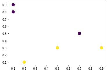
In the figure below, we can see the data which we have created. By looking at it we can say that the data is linearly separable and can be solvable using a perceptron network. Since the motive of the article is to visualize the process of the network, it will be a better approach to use only two parameters in the network. Visualizing the training of such parameters can provide us with great explainability.
import matplotlib.pyplot as plt

plt.scatter(X[:, 0], X[:, 1], c=y, s=100)
plt.show()
The below code is a representation of the error rate. The error rate is dependent on the weights of the network. As the error rate decreases, accuracy in results increases.
default_weight = np.array([[-4.], [-4.]])
In the code, we can see that we have chosen (-4, -4) points, because as we move to the left side we will get a bad result from the network. Bad results from the network make the explainability of the network increase. In this article, we will try to make the network’s error smaller. Every network starts at a place with coordinates (-4, -4) and finishes near the point with the lower error.
After defining the error rate we are required to initialize a contour so that we can draw the procedure of every backpropagation algorithm. The below code can help us on initializing a contour:
plt.title("Approximation function contour plot")
plt.xlabel("First weight")
plt.ylabel("Second weight")
draw_countour(
    np.linspace(-5, 5, 50),
    np.linspace(-5, 5, 50),
    network_target_function
)
Output:
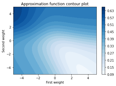
In this article, we are not posting the whole code of the procedure. Any interested reader can check the whole code here. Still, before going on the main motive we are required to know about the functions which we have defined to complete the process. The function list is below:
- Draw contour: In the above, we have seen the contour function which will help in plotting the procedure of backpropagation algorithms.
- Weights quiver and save epoch weights functions are there that will help in procuring weights and a signal processor which saves weight updates for every epoch.
- Function for network creation that can help in generating a new network every time we call it.
- Draw quiver can help in the Train algorithm and draw quiver for every epoch update for this algorithm.
The below list represents the 5 topmost backpropagation algorithms:
- Gradient descent
- Momentum
- Rprop
- iRprop+
- Gradient Descent + Golden Search
Now we can start by visualizing these algorithms one by one. We will start from gradient descent.
Gradient descent
Gradient descent can be defined as an optimization algorithm where it follows the iterative method to find the minima or maxima of any function. We commonly use it to minimize the cost function. Here we will use it to minimize our error rate.
After defining all the functions we can call them for minimizing the error rate using the gradient descent method. The below code can help us with this.
algorithms = (
    (partial(algorithms.GradientDescent, step=0.3), 'Gradient Descent', 'k'),
)

patches = []
for algorithm, algorithm_name, color in algorithms:
    print("The '{}' network training".format(algorithm_name))
    quiver_patch = draw_quiver(algorithm, algorithm_name, color)
    patches.append(quiver_patch)

print("Plot training results")
plt.legend(handles=patches)
plt.show()
Output:
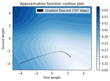
In the above plot, we can see that we get a value close to 0.125 where the procedure uses the 797 steps. That curve is a representation of steps followed by the gradient descent algorithm.
Momentum
Momentum is also a very popular backpropagation algorithm and when applied in the network it works with a concept which states that previous changes in the weights should influence the current direction of movement in weight space which means once the weights start moving in a particular direction in weight space, they tend to continue moving in that direction. We can visualize the process using the following code.
algorithms = (
    (partial(algorithms.Momentum, batch_size=None, step=0.3), 'Momentum', 'g'),
)

patches = []
for algorithm, algorithm_name, color in algorithms:
    print("The '{}' network training".format(algorithm_name))
    quiver_patch = draw_quiver(algorithm, algorithm_name, color)
    patches.append(quiver_patch)

print("Plot training results")
plt.legend(handles=patches)
plt.show()
Output:

In the visualization of this algorithm for backpropagation, we can see that we again reach closer to the 0.125 from (-4,-4) and the steps this algorithm has gone through are 92 and also we can see the proof that in this algorithm the gradient stars changing its direction weight update vector magnitude will decrease.
Rprop
Rprop stands for resilient backpropagation. This algorithm computes updates of the weight by using the sign of gradient. Basically, it adapts the step size in a dynamic nature for each weight. We can understand it more by visualizing the nature of work in backpropagation. We can do this using the following codes.
algorithms = (
    (partial(algorithms.RPROP, step=0.3), 'RPROP', 'm'),
)

patches = []
for algorithm, algorithm_name, color in algorithms:
    print("The '{}' network training".format(algorithm_name))
    quiver_patch = draw_quiver(algorithm, algorithm_name, color)
    patches.append(quiver_patch)

print("Plot training results")
plt.legend(handles=patches)
plt.show()
Output:
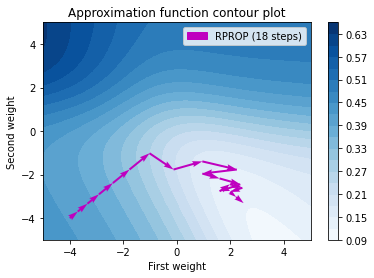
In the above visualization, we can see that the number of steps is very less than the above methods and also it proves that it adapts the step size in a dynamic nature for each weight independently.
iRprop+
This algorithm can be considered as an improvement in Rprop algorithms. We use it to make the backpropagation faster than the other algorithms with a lower amount of steps. Visualization of this algorithm can be performed using the following codes.
algorithms = (
    (partial(algorithms.IRPROPPlus, step=0.3), 'iRPROP+', 'r'),
)

patches = []
for algorithm, algorithm_name, color in algorithms:
    print("The '{}' network training".format(algorithm_name))
    quiver_patch = draw_quiver(algorithm, algorithm_name, color)
    patches.append(quiver_patch)

print("Plot training results")
plt.legend(handles=patches)
plt.show()
Output:

In the above output, we can see that the number of steps in backpropagation is lower than in the Rprop algorithms. Also, the first few steps are similar to the Rprop algorithms.
Gradient Descent and Golden Search
This algorithm can not be considered as an independent algorithm for backpropagation. It requires other methods to be added to it for backpropagation. We use this method to reduce the number of methods but sometimes it becomes time-consuming because it searches for the optimal step to be taken for finding the minimum error rate. We can visualize the procedure of this algorithm using the following code:
algorithms = (
    (partial(algorithms.Hessian, penalty_const=0.01), "Newton's method", 'y'),
)

patches = []
for algorithm, algorithm_name, color in algorithms:
    print("The '{}' network training".format(algorithm_name))
    quiver_patch = draw_quiver(algorithm, algorithm_name, color)
    patches.append(quiver_patch)

print("Plot training results")
plt.legend(handles=patches)
plt.show()
Output:
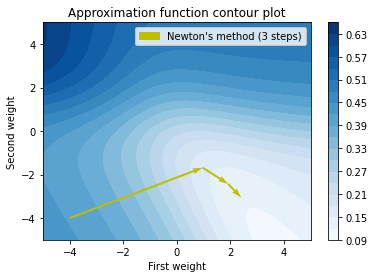
In the above code, we can see that we used gradient descent with this algorithm. In the above when we used gradient descent alone we found that the completion of the process took around 197 steps and here we can see that similar results we get in 3 steps because of this algorithm.
We can also combine these algorithms together for comparison.
In the above visualization, we can see the procedure and results from all the above-given algorithms.
Final words
In this article, we have seen how the backpropagation algorithm can be visualized to make them more explainable. Along with this, we have also drawn a combined visualization so that we can compare the results and procedure of all the algorithms to find a minimum error rate.


