Rendering, also known as image synthesis, generates an output from a set of specific descriptions. It can also be described as transforming an impression or idea into a real space. Rendering Systems find their application in a wide spectrum of areas and across a variety of industries. Rendering these days is used in architecture, video games, simulators, movie and TV Visual effects and design visualization. It can be used to figure out the final layout for housing architecture, visualize what a final product might look like in the manufacturing industry and much more. One popular such use case for Rendering can be found in Image Processing. By using Rendering techniques, the description of an image is transformed into an actual image. For delivering the output, computational power is taught and used as a tool. Photorealistic and Non Photorealistic images can be implemented using 2D and 3D modelling techniques.
The resulting output image is called a “render”. A model is created to execute the rendering process, and multiple such models can be defined to create a scene file, a file with predefined objects presented in a data structure. The data contained in the scene file is then passed through a rendering program to be processed and generated output in a digital image or graphical image file. Image Rendering is an essential step for graphical pipelines as they provide mere models with their final appearance. Metrics like viewpoint, texture, lighting and shading can be easily adjusted during the synthesis. With the rapid development of computational power, it has become one of the most hotly debated areas of implementation.
As a product, a wide variety of renderers are available in the market. Some are integrated into larger modelling programs and animation packages, while some are stand-alone, others being free and open-source projects. When the pre-image or the borderline wireframe sketch gets completed, rendering is used, adding in the bitmap and procedural textures, lights, mapping, and relative positioning to the objects in the image being processed. The result is a completed image the consumer or intended viewer sees.
There are a few different types of efficient modelling techniques that have emerged: rasterization, which includes scanline rendering, considers the objects in the scene and projects them to form an image; ray casting technique considers the scene as observed from a specific point-of-view and calculates the observed image based only on its geometry and provides judgement based on very basic optical laws of reflection intensity, also using Monte Carlo technique to reduce artifacts. The Monte Carlo technique is used in most, to obtain more realistic results at a speed that is often orders of magnitude slower.
What is AutoInt?
AutoInt, also known as Automatic integration, is a modern image rendering library used for high volume rendering using deep neural networks. It is used to learn closed-form solutions to an image volume rendering equation, an integral equation that accumulates transmittance and emittance along rays to render an image. While conventional neural renderers require hundreds of samples along each ray to evaluate such integrals and require hundreds of costly forward passes through a network, AutoInt allows evaluating these integrals with far fewer forward passes.
For training, it first instantiates the computational graph corresponding to the derivative of the coordinate-based network. The graph is then fitted to the signal to integrate. After optimization, it reassembles the graph to obtain a network that represents the antiderivative. Using the fundamental theorem of calculus enables the calculation of any definite integral in two evaluations of the network. By applying such an approach to neural image rendering, the tradeoff between rendering speed and image quality is improved on a greater scale, in turn improving render times by greater than 10× with a tradeoff of slightly reduced image quality.
The AutoInt Framework
The AutoInt Framework is distributed into four essential parts :
- A predefined integral network architecture that instantiates the integral network.
- Building the corresponding grad network, which is later.
- Optimized to represent a function.
- Definite integrals can then be computed by evaluating the integral network, which shares parameters with its grad network.

During training in the volume rendering pipeline, the grad networks representing volume density through σ and the color c are optimized for a given set of multi-view images. For inference synthesis, the grad networks’ parameters are reassembled to form the integral networks, representing antiderivatives that can be efficiently evaluated to calculate the ray integrals through the volume. A sampling network then predicts the locations of piecewise sections used for evaluating the definite integrals.
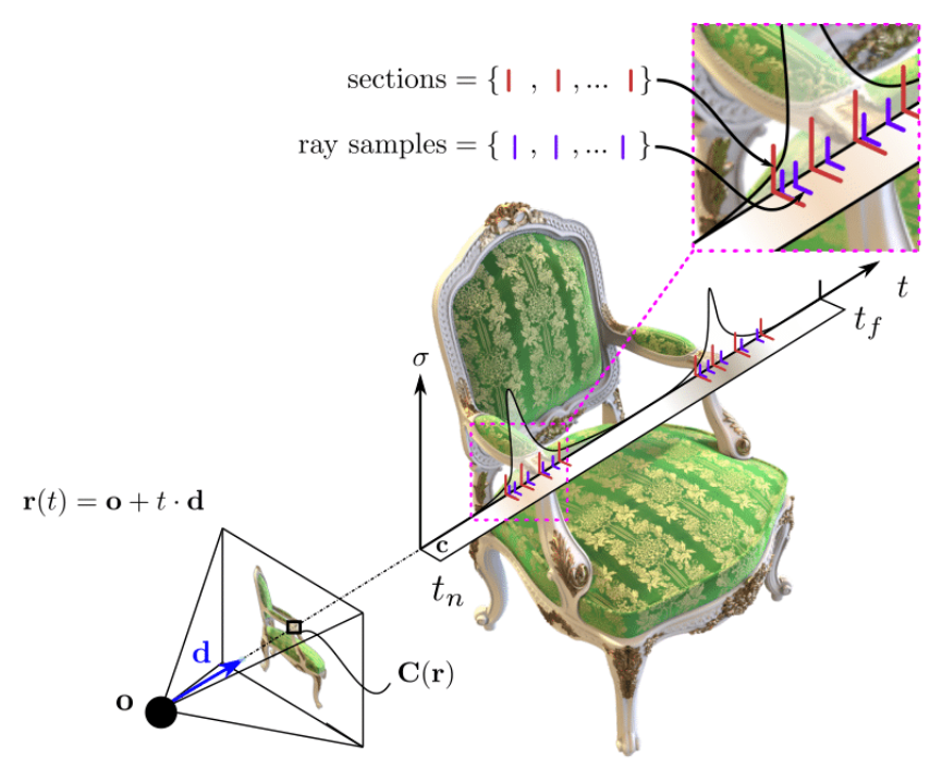
The grad network is then fit to the input image signal with direct supervision. The integral network is now reassembled, and querying the output results in a 1D signal that is integral to the input coordinate.
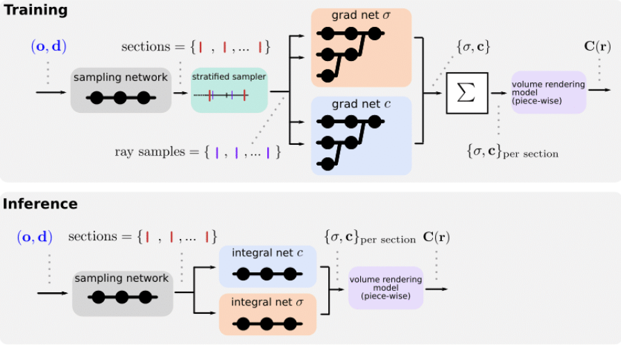
AutoInt uses piecewise approximation to learn efficient closed-form solutions to integrals from the input image signals along sections. At the time of inference, rather than using hundreds of forwarding passes, it evaluates the signals efficiently using piecewise division along the ray. The rendered piecewise sections result in high image quality generated.

Implementing AutoInt
We will try to implement an example of AutoInt where we will first create class coordinates on a sample 1D function we wish to fit. We will infuse different functions we want to integrate, after which we will try to set up the integral and grad network and finally fit our grad network on the integral function. So let’s get started.
Installing the AutoInt Libraries
We will first import and install a bunch of third party libraries to get started with. We will use torchmeta here, a collection of extensions and data-loaders for few-shot learning & meta-learning in PyTorch. Torchmeta contains popular meta-learning benchmarks to use.
The following is an official implementation from AutoInt’s tutorial, the link to the colab notebook can be found here.
#installing dependencies
 import torch
 import matplotlib.pyplot as plt
 import numpy as np
 from functools import partial
 from torch.utils.data import DataLoader
 !pip install --no-dependencies torchmeta==1.4.6
 !pip install ordered-set
 !pip install colour
 from torchmeta.modules import MetaModule
Importing the AutoInt Library,
 import sys
 import os
 from autoint.session import Session
 import autoint.autograd_modules as autoint
Getting Started
Creating A class to create coordinates from a 1D function we wish to fit.
 #creating a class for 1D functions to fit
 class Implicit1DWrapper(torch.utils.data.Dataset):
     def __init__(self, range, fn, grad_fn=None, integral_fn=None, sampling_density=100,
                  train_every=10):
         avg = (range[0] + range[1]) / 2
         coords = self.get_samples(range, sampling_density)
         self.fn_vals = fn(coords)
         self.train_idx = torch.arange(0, coords.shape[0], train_every).float()
         #coords = (coords - avg) / (range[1] - avg)
         self.grid = coords
         self.grid.requires_grad_(True)
         #self.val_grid = val_coords
         if grad_fn is None:
             grid_gt_with_grad = coords
             grid_gt_with_grad.requires_grad_(True)
             fn_vals_with_grad = fn((grid_gt_with_grad * (range[1] - avg)) + avg)
             gt_gradient = torch.autograd.grad(fn_vals_with_grad, [grid_gt_with_grad],
                                               grad_outputs=torch.ones_like(grid_gt_with_grad), create_graph=True,
                                               retain_graph=True)[0]
             try:
                 gt_hessian = torch.autograd.grad(gt_gradient, [grid_gt_with_grad],
                                                  grad_outputs=torch.ones_like(gt_gradient), retain_graph=True)[0]
             except Exception as e:
                 gt_hessian = torch.zeros_like(gt_gradient)
         else:
             gt_gradient = grad_fn(coords)
             gt_hessian = torch.zeros_like(gt_gradient)
         self.integral_fn = integral_fn
         if integral_fn:
             self.integral_vals = integral_fn(coords)
         self.gt_gradient = gt_gradient.detach() #implementing gradient
         self.gt_hessian = gt_hessian.detach()
     def get_samples(self, range, sampling_density):
         num = int(range[1] - range[0])*sampling_density
         avg = (range[0] + range[1]) / 2
         coords = np.linspace(start=range[0], stop=range[1], num=num)
         coords.astype(np.float32)
         coords = torch.Tensor(coords).view(-1, 1)
         return coords
     def get_num_samples(self):
         return self.grid.shape[0]
     def __len__(self):
         return 1
     def __getitem__(self, idx):
         if self.integral_fn is not None:
             return {'coords':self.grid}, {'integral_func': self.integral_vals, 'func':self.fn_vals,
                     'gradients':self.gt_gradient, 'val_func': self.val_fn_vals,
                     'val_coords': self.val_grid, 'hessian':self.gt_hessian}
         else:
             return {'idx': self.train_idx, 'coords':self.grid}, \
                    {'func': self.fn_vals, 'gradients':self.gt_gradient,
                     'coords': self.grid}
 Defining the different 1D functions we want to integrate in our network,
 #integrating different 1D Functions
 def cos_fn(coords):
   return torch.cos(10*coords)
 def polynomial_fn(coords):
     return .1*coords**5 - .2*coords**4 + .2*coords**3 - .4*coords**2 + .1*coords
 def sinc_fn(coords):
     coords[coords == 0] += 1
     return torch.div(torch.sin(20*coords), 20*coords)
 def linear_fn(coords):
     return 1.0 * coords
 def xcosx_fn(coords):
     return coords * torch.cos(coords)
 def integral_xcosx_fn(coords):
     return coords*torch.sin(coords) + torch.cos(coords)
We will now set up the integral network and the grad network; we will first define an integral network using the AutoInt API. Here the integral network is an MLP with sine non-linearities: a SIREN.
 #creating the SIREN class and defining the structure
 class SIREN(MetaModule):
     def __init__(self, session):
         super().__init__()
         self.net = []
         self.input = autoint.Input(torch.Tensor(1, 1), id='x_coords')
         self.net.append(autoint.Linear(1, 128))
         self.net.append(autoint.Sine())
         self.net.append(autoint.Linear(128, 128))
         self.net.append(autoint.Sine())
         self.net.append(autoint.Linear(128, 128))
         self.net.append(autoint.Sine())
         self.net.append(autoint.Linear(128, 128))
         self.net.append(autoint.Sine())
         self.net.append(autoint.Linear(128, 1))
         self.net = torch.nn.Sequential(*self.net)
         self.session = session
     def input_init(self, input_tensor, m):
         with torch.no_grad():
             if isinstance(m, autoint.Input):
                 m.set_value(input_tensor, grad=True)
     def constant_init(self, input_tensor, m):
         with torch.no_grad():
             if isinstance(m, autoint.Constant):
                 m.set_value(input_tensor, grad=False)
     def forward(self, x):
         with torch.no_grad():
             input_init_func = partial(self.input_init, x[:, 0, None])
             self.input.apply(input_init_func)
         input_ctx = autoint.Value(x, self.session)
         out1 = self.input(input_ctx)
         return self.net(out1)
In AutoInt, a session helps handle the derivation of the integral network into the grad network. It also takes care of the reassembly of the weights too.
integralnet_session = Session() #creating session
Instantiating the integral net, we defined earlier. Thus, the session can be thought of as representing the integral network.
 #instantiate the integral network using cuda
 net = SIREN(integralnet_session)
 net.cuda()
We will get the following output,
 SIREN(
   (input): Input()
   (net): Sequential(
     (0): Linear()
     (1): Sine()
     (2): Linear()
     (3): Sine()
     (4): Linear()
     (5): Sine()
     (6): Linear()
     (7): Sine()
     (8): Linear()
   )
   (session): Session()
 )
We can evaluate the SIREN we instantiated using the forward function as we would do for any Pytorch module.
 x = torch.ones(1, 1).cuda() # defines a dummy input
 y = torch.ones(1, 1).cuda()
 x.requires_grad_(True)
 session_input = {'x_coords': x,
                  #'y_coords': y,
                  'params': None}
 y = net(x)
 forward_siren_evaluation = y.data #print result of evaluation
 print(f"result of forward SIREN evaluation={forward_siren_evaluation}")
Output :
result of forward SIREN evaluation=tensor([[0.0843]], device='cuda:0', grad_fn=<AddBackward0>)
We can now visualize the integral network we created by visualizing its associated session :
integralnet_session.draw() #visualizing the integral network

gradnet_session.draw() #visualzing gradnet

Fitting the grad network
We first choose the function we want to calculate the integral using AutoInt.
func_to_fit = cos_fn #using cos function
We create the data loader that will create the pairs of data points of the form (input coordinate, output of the function to integrate).
 dataset = Implicit1DWrapper([-1,1], fn=func_to_fit, \
                             sampling_density=1000, train_every=1)
 dataloader = DataLoader(dataset,shuffle=True, batch_size=1, \
                         pin_memory=True, num_workers=0)
 def dict2cuda(d):
     tmp = {}
     for key, value in d.items():
         if isinstance(value, torch.Tensor):
             tmp.update({key: value.cuda()})
         else:
             tmp.update({key: value})
     return tmp
Training loop to fit the function for 500 epochs and Adam Optimizer :
 epochs = 500 #setting the number of epochs
 loss_fn = torch.nn.MSELoss() #setting loss function
 optimizer = torch.optim.Adam(lr=5e-5, params=net.parameters(),amsgrad=True) #setting optimizer
 print_loss_every = 50
 for e in range(epochs):
   for step, (input, gt) in enumerate(dataloader):
       input = dict2cuda(input)
       gt = dict2cuda(gt)
       gradnet_output = gradnet_session.compute_graph_fast({'x_coords': input['coords'],
                                                            'params': None})
       loss = loss_fn(gradnet_output,gt['func']).mean()
       optimizer.zero_grad()
       loss.backward()
       optimizer.step()
   if not e % print_loss_every:
       print(f"{e}/{epochs}: loss={loss}")
 0/500: loss=0.5242253541946411
 50/500: loss=0.0002673180715646595
 100/500: loss=8.674392120155971e-06
 150/500: loss=3.343612206663238e-06
 200/500: loss=2.0269669676054036e-06
 250/500: loss=1.393691377415962e-06
 300/500: loss=1.0891841384363943e-06
 350/500: loss=9.32661862407258e-07
 400/500: loss=0.0003990948316641152
 450/500: loss=7.659041330043692e-06
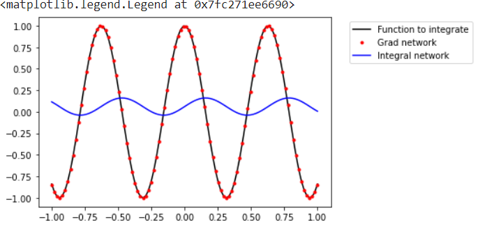
Plotting results using matplotlib :
 #plotting our results
 x_coords = torch.linspace(-1,1,100)[:,None].cuda()
 grad_vals = func_to_fit(x_coords).cpu()
 fitted_grad_vals = gradnet_session.compute_graph_fast({'x_coords': x_coords,
                                                        'params': None}).cpu()
 integral_vals = integralnet_session.compute_graph_fast({'x_coords': x_coords,
                                                         'params': None}).cpu()
 x_coords = x_coords.cpu()
 plt.plot(x_coords,grad_vals,'-k', label='Function to integrate')
 plt.plot(x_coords,fitted_grad_vals.detach(),'.r', label='Grad network')
 plt.plot(x_coords,integral_vals.detach(),'-b', label='Integral network')
 plt.legend(bbox_to_anchor=(1.05, 1.0), loc='upper left')
EndNotes
This article talks about how the image rendering library AutoInt works and tries to get a hands-on overview of what happens under the hood when the input signals process. I would recommend exploring the library even further using other modules to understand its immense qualities even better. You can access my implemented colab notebook here.
Happy Learning!


