Modern machine learning or one can say deep learning algorithms, have become really good at multiple tasks. For example, object detection tasks have been overtaken by modern ML methods.
There is a growing understanding that larger models are “easy” to optimise in the sense that local methods, such as stochastic gradient descent (SGD), converge to global minima of the training risk in over-parameterized regimes. Thus, it is believed that large interpolating models can have low test risk and be easy to optimise at the same time.
Appropriately chosen “modern” models usually outperform the optimal “classical” model on the test set. Another important practical advantage of over-parameterized models is in optimisation.
However, it is now common practice to fit highly complex models like deep neural networks to data with (nearly) zero training error, and yet these interpolating predictors are observed to have good out-of-sample accuracy even for noisy data.
Overview Of Bias-Variance Trade-Offs In ML
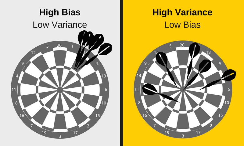
Source: elitedatascience
Bias is the difference between the model’s expected predictions and the true values and variance refers to the algorithm’s sensitivity to specific sets of training data. Bias vs. variance refers to the accuracy vs. consistency of the models trained by the algorithm.
To build a good predictive model, one needs to find a balance between bias and variance that minimises the total error because:
Total Error = Bias^2 + Variance + Irreducible Error
An optimal balance of bias and variance leads to a model that is neither overfitting nor underfitting. The predictor is commonly chosen from linear functions or neural networks with a certain architecture, using empirical risk minimisation (ERM) and its variants.
Bridging The Old And New

The classical approach to understanding generalisation is based on bias-variance trade-offs, where model complexity is carefully calibrated so that they fit on the training sample reflects performance out-of-sample.
In an attempt to investigate the bias-variance tradeoff for neural networks and to shed more light on their generalisation properties, researchers at Ohio State University and Columbia University, by introducing a new “double descent” risk curve that extends the traditional U-shaped bias-variance curve beyond the point of interpolation.
The experimental results show that while the behaviour of SGD for more general neural networks are not fully understood, there is significant empirical and some theoretical evidence that a similar minimum norm inductive bias is present and averaging potentially non-smooth interpolating solutions leads to an interpolating solution with a higher degree of smoothness.
Above picture has a classical U-shaped risk curve arising from the bias-variance trade-off on the left and a e double descent risk curve, which incorporates the U-shaped risk curve (i.e., the “classical” regime) together with the observed behavior from using high complexity function classes (i.e., the “modern” interpolating regime) on the right.
The belief that a model with zero training error is overfit to the training data and will typically generalise poorly is very popular amongst ML practitioners. However, modern machine learning methods, nowadays, fit the training data perfectly or near-perfectly. For instance, highly complex neural networks and other non-linear predictors are often trained to have very low or even zero training risk.
In spite of the high function class complexity and near-perfect fit to the training data, these predictors often give accurate predictions on new data.
This attempt to bridge the two regimes through fundamental statistics standpoint is to maintain the intuition around machine learning models intact.
Evolution On Other Fronts

As we discuss something as fundamental as reconciling bias-variance trade-offs in modern ML methods, research is being done in some unheard avenues. Questions such as whether backpropagation is necessary and what is the importance of feedback loops for recommendation engines are being asked. Robustness of a machine learning model is being achieved by introducing noise during training. Researchers have gone as far as preparing a model to train better. In short, energies are shifting from post-training and testing to pre-training strategies.
The algorithms get tweaked for trivialities every other day. The errors too, have kept on advancing. For instance, it has been demonstrated that reinforcement learning models can run into reward hacking problem out of nowhere. While it is obvious that the apple has indeed fallen from the tree, traditional approaches still hold significance because one doesn’t always have to fancy too many deep learning layers or pre-trained BERT for something as simple as document classification!
However, techniques like Yolo net take the image as input and provide the location and name of objects at the output. But in traditional ones like SVM, a bounding box object detection algorithm is required first to identify all possible objects to have the HOG(histogram of oriented gradients) as input to the learning algorithm in order to recognise relevant objects.
The histogram of oriented gradients (HOG) is a feature descriptor used in computer vision and image processing for the purpose of object detection. Feature descriptors describe elementary characteristics such as the shape, the colour, the texture or the motion, among others.
Though setting up a deep learning project uses up more resources than a typical SVMs(support vector machines), they are really good at dealing with complex problems. Problems which have more features.