The Deep Convolutional Neural Network has variants applied as transfer learning frameworks. In the transfer learning approach, these models can be used with the pre-trained weights on the ImageNet dataset. In one of our previous articles, we have implemented the VGG16, VGG19 and ResNet50 models in image classification. We have also discussed and implemented the ALexNet model in the same task and compared the performance of all the above models. Here, we are going to discuss the MobileNet and ResNet-50 models which are the light architectures of Deep Convolutional Neural Network.
In this article, we will compare the MobileNet and ResNet-50 architectures of the Deep Convolutional Neural Network. First, we will implement these two models in CIFAR-10 classification and then we will evaluate and compare both of their performances and with other transfer learning models in the same task.
MobileNet
The MobileNet was proposed as a deep learning model by Andrew G. Howard et al of Google Research team in their research work entitled “MobileNets: Efficient Convolutional Neural Networks for Mobile Vision Applications”. This model was proposed as a family of mobile-first computer vision models for TensorFlow, designed to effectively maximize accuracy while being mindful of the restricted resources for an on-device or embedded application. MobileNets are small, low-latency, low-power models parameterized to meet the resource constraints of a variety of use cases. They can be built upon for classification, detection, embedding and segmentation similar to how other popular large scale models.
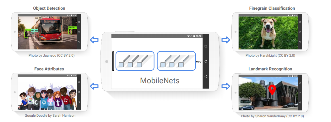
(Image Source: Original Research Paper)
ResNet-50
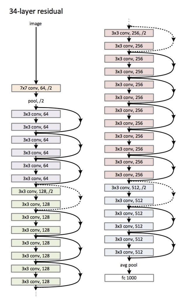
ResNet-50 is a convolutional neural network that is 50 layers deep. You can load a pre-trained version of the network trained on more than a million images from the ImageNet database. The pre-trained network can classify images into 1000 object categories, such as a keyboard, mouse, pencil, and many animals. As a result, the network has learned rich feature representations for a wide range of images. The architecture of a ResNet-50 model can be given in the below figure.
Implementation
Before implementing the above models, we will download and preprocess the CIFAR-10 dataset. All the steps will be the same as we have done in the previous articles.
#Keras library for CIFAR dataset from keras.datasets import cifar10 (x_train,y_train),(x_test,y_test)=cifar10.load_data() W_grid=5 L_grid=5 fig,axes = plt.subplots(L_grid,W_grid,figsize=(10,10)) axes=axes.ravel() n_training=len(x_train) for i in np.arange(0,L_grid * W_grid): index=np.random.randint(0,n_training) #Pick a random number axes[i].imshow(x_train[index]) axes[i].set_title(y_train[index]) #Prints labels on top of the picture axes[i].axis('off') plt.subplots_adjust(hspace=0.4)#Split x_train,x_val,y_train,y_val=train_test_split(x_train,y_train,test_size=.3) #Dimension of the CIFAR10 dataset print((x_train.shape,y_train.shape)) print((x_val.shape,y_val.shape)) print((x_test.shape,y_test.shape))
#Onehot Encoding the labels. #Since we have 10 classes we should expect the shape[1] of y_train,y_val and y_test to change from 1 to 10 y_train=to_categorical(y_train) y_val=to_categorical(y_val) y_test=to_categorical(y_test) #Verifying the dimension after onehot encoding print((x_train.shape,y_train.shape)) print((x_val.shape,y_val.shape)) print((x_test.shape,y_test.shape))
#Image Data Augmentation train_generator = ImageDataGenerator(rotation_range=2, horizontal_flip=True, zoom_range=.1 ) val_generator = ImageDataGenerator(rotation_range=2, horizontal_flip=True,zoom_range=.1) test_generator = ImageDataGenerator(rotation_range=2, horizontal_flip= True, zoom_range=.1) #Fitting the augmentation defined above to the data train_generator.fit(x_train) val_generator.fit(x_val) test_generator.fit(x_test) #Learning Rate Annealer lrr= ReduceLROnPlateau(monitor='val_accuracy', factor=.01, patience=3, min_lr=1e-5)
Implementation of ResNet-50
Now, as we are ready with the data set, we will implement the first model that is ResNet-50.
#Instantiating ResNet50 base_model_resnet = ResNet50(include_top=False,weights='imagenet',input_shape=(32,32,3),classes=y_train.shape[1]) #Defining and Adding layers model_resnet=Sequential() #Add the Dense layers along with activation and batch normalization model_resnet.add(base_model_resnet) model_resnet.add(Flatten()) #Add the Dense layers along with activation and batch normalization model_resnet.add(Dense(1024,activation=('relu'),input_dim=512)) model_resnet.add(Dense(512,activation=('relu'))) model_resnet.add(Dropout(.4)) model_resnet.add(Dense(256,activation=('relu'))) model_resnet.add(Dropout(.3))#Adding a dropout layer that will randomly drop 30% of the weights model_resnet.add(Dense(128,activation=('relu'))) model_resnet.add(Dropout(.2)) model_resnet.add(Dense(10,activation=('softmax'))) #This is the classification layer #Model summary model_resnet.summary()#Defining the parameters batch_size= 100 epochs=30 learn_rate=.001 sgd=SGD(lr=learn_rate,momentum=.9,nesterov=False) #Compile model_resnet.compile(optimizer=sgd,loss='categorical_crossentropy',metrics=['accuracy']) #Training model_resnet.fit_generator(train_generator.flow(x_train,y_train,batch_size=batch_size), epochs=epochs, steps_per_epoch=x_train.shape[0]//batch_size, validation_data=val_generator.flow(x_val,y_val,batch_size=batch_size),validation_steps=250,callbacks=[lrr],verbose=1)

#Plotting the training and validation loss f,ax=plt.subplots(2,1) #Creates 2 subplots under 1 column #Assigning the first subplot to graph training loss and validation loss ax[0].plot(model_resnet.history.history['loss'],color='b',label='Training Loss') ax[0].plot(model_resnet.history.history['val_loss'],color='r',label='Validation Loss') #Plotting the training accuracy and validation accuracy ax[1].plot(model_resnet.history.history['accuracy'],color='b',label='Training Accuracy') ax[1].plot(model_resnet.history.history['val_accuracy'],color='r',label='Validation Accuracy')
#Making prediction y_pred3=model_resnet.predict_classes(x_test) y_true=np.argmax(y_test,axis=1) #Defining function for confusion matrix plot def plot_confusion_matrix(y_true, y_pred, classes, normalize=False, title=None, cmap=plt.cm.Blues): if not title: if normalize: title = 'Normalized confusion matrix' else: title = 'Confusion matrix, without normalization' # Compute confusion matrix cm = confusion_matrix(y_true, y_pred) if normalize: cm = cm.astype('float') / cm.sum(axis=1)[:, np.newaxis] print("Normalized confusion matrix") else: print('Confusion matrix, without normalization') # print(cm) fig, ax = plt.subplots(figsize=(7,7)) im = ax.imshow(cm, interpolation='nearest', cmap=cmap) ax.figure.colorbar(im, ax=ax) # We want to show all ticks... ax.set(xticks=np.arange(cm.shape[1]), yticks=np.arange(cm.shape[0]), # ... and label them with the respective list entries xticklabels=classes, yticklabels=classes, title=title, ylabel='True label', xlabel='Predicted label') # Rotate the tick labels and set their alignment. plt.setp(ax.get_xticklabels(), rotation=45, ha="right", rotation_mode="anchor") # Loop over data dimensions and create text annotations. fmt = '.2f' if normalize else 'd' thresh = cm.max() / 2. for i in range(cm.shape[0]): for j in range(cm.shape[1]): ax.text(j, i, format(cm[i, j], fmt), ha="center", va="center", color="white" if cm[i, j] > thresh else "black") fig.tight_layout() return ax np.set_printoptions(precision=2) #Plotting the confusion matrix confusion_mtx=confusion_matrix(y_true,y_pred3) class_names=['airplane', 'automobile', 'bird', 'cat', 'deer', 'dog', 'frog', 'horse', 'ship', 'truck'] # Plotting non-normalized confusion matrix plot_confusion_matrix(y_true, y_pred3, classes=class_names, title='Non-Normalized ResNet50 Confusion Matrix')
# Plotting normalized confusion matrix plot_confusion_matrix(y_true, y_pred3, classes=class_names, normalize=True, title='Normalized ResNet50 Confusion Matrix')
from sklearn.metrics import accuracy_score resnet_acc = accuracy_score(y_true, y_pred3) print('Accuracy Score of ResNet50 = ', resnet_acc)

Implementing MobileNet
from keras.applications import MobileNet #Adding the final layers to the above base models where the actual classification is done in the dense layers model_mobnet = Sequential() model_mobnet.add(base_MobNet) model_mobnet.add(Flatten()) model_mobnet.add(Dense(1024,activation=('relu'),input_dim=512)) model_mobnet.add(Dense(512,activation=('relu'))) model_mobnet.add(Dense(256,activation=('relu'))) #model_mobnet.add(Dropout(.3)) model_mobnet.add(Dense(128,activation=('relu'))) #model_mobnet.add(Dropout(.2)) model_mobnet.add(Dense(10,activation=('softmax'))) # Model Summary model_mobnet.summary()#Compiling the MobileNet model model_mobnet.compile(optimizer=sgd,loss='categorical_crossentropy',metrics=['accuracy']) #Training model_mobnet.fit_generator(train_generator.flow(x_train, y_train, batch_size = batch_size), epochs=100, steps_per_epoch = x_train.shape[0]//batch_size, validation_data = val_generator.flow(x_val, y_val, batch_size = batch_size), validation_steps = 250, callbacks = [lrr], verbose = 1)

#Plotting the training and validation loss f,ax=plt.subplots(2,1) #Creates 2 subplots under 1 column #Training loss and validation loss ax[0].plot(model_mobnet.history.history['loss'],color='b',label='Training Loss') ax[0].plot(model_mobnet.history.history['val_loss'],color='r',label='Validation Loss') #Training accuracy and validation accuracy ax[1].plot(model_mobnet.history.history['accuracy'],color='b',label='Training Accuracy') ax[1].plot(model_mobnet.history.history['val_accuracy'],color='r',label='Validation Accuracy')
#Making prediction y_pred2 = model_mobnet.predict_classes(x_test) #Plotting the confusion matrix confusion_mtx=confusion_matrix(y_true,y_pred2) class_names=['airplane', 'automobile', 'bird', 'cat', 'deer', 'dog', 'frog', 'horse', 'ship', 'truck'] #Plotting non-normalized confusion matrix plot_confusion_matrix(y_true, y_pred2, classes = class_names, title = 'Non-Normalized MobileNet Confusion Matrix')
#Plotting normalized confusion matrix plot_confusion_matrix(y_true, y_pred2, classes = class_names, normalize = True, title = 'Normalized MobileNet Confusion matrix')
#Accuracy of MobileNet from sklearn.metrics import accuracy_score acc2 = accuracy_score(y_true, y_pred2) print('Accuracy Score of MobileNet = ', acc2)

As we can see in the confusion matrices and average accuracies, ResNet-50 has given better accuracy than MobileNet. The ResNet-50 has accuracy 81% in 30 epochs and the MobileNet has accuracy 65% in 100 epochs. But as we can see in the training performance of MobileNet, its accuracy is getting improved and it can be inferred that the accuracy will certainly be improved if we run the training for more number of epochs. However, we have shown the architecture and way to implement both the models. ResNet-50 has more number of parameters to be used so it is obvious that it will show better performance as compared to the MobileNet.


