This article gives us a brief overview of the most used loss functions to optimize machine learning algorithms. We all use machine learning algorithms to solve various complex problems and select them based on the loss function value and evaluation metrics. But do we know that we are selecting the correct loss function for our algorithm? If not, then let’s find out.

Mainly the loss functions are divided into three categories:

Regression loss functions

1. Mean Squared Error
2. Mean Squared Logarithmic Error
3. Mean Absolute Error
4. Binary classification loss functions

Binary Cross Entropy

1. Hinge Loss
2. Squared Hinge Loss

Multi-class classification loss functions 

1. Multi-class cross entropy
2. Sparse multi-class cross entropy 
3. Kullback Leibler divergence loss

What are loss functions?

Loss functions (also known as objective functions) are equations that give you a curve of loss generated by the predictions of your model. Our aim is to minimize the loss function to enhance the accuracy of the model for better predictions. Now that we know what a loss function is, let’s see which loss function to use when.

Regression loss functions:

There are plenty of regression algorithms like linear regression, logistic regression, random forest regressor, support vector machine regressor etc. and all the algorithms require loss functions to make it converge better.

• Mean Squared Error (MSE):

This is one of the most popular and well-known loss functions. Also known as L2 loss. It’s simple yet very powerful and helps you understand how well your model is performing. Below is the formula to calculate the MSE. 

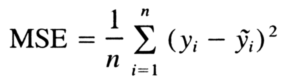
It is the average of the difference between the true value and the predicted value for all predictions made by the algorithm. In other words, it is the squared average of all errors. Higher value of MSE signifies that the model hasn’t learned efficiently.

• Mean Squared Logarithmic Error (MSLE):

This is a variant of the MSE. Here we take log of true and predicted values and find out the ratio. There are some advantages of using MSLE. MSLE doesn’t penalize the large error significantly more than the small ones, especially when the target variable has large values. One more thing to be kept in mind is that MSLE should be used with continuous data for better results.

The above given is the formula to calculate MSLE for regression. We also talked about the ratio, which is nothing but a simple logarithmic property.

And if you notice carefully, besides log we are also adding 1 to the predicted and true value. Sometimes either the true or the predicted value can be zero and log(zero) is not defined, so we have to add one to make sure that the equation is solvable. MSLE helps you separate the penalties for overestimates and underestimates whereas there is no categorization in MSE. MSLE penalizes underestimates more than overestimates.

• Mean Absolute Error (MAE):

MAE or L1 loss gives us a non-directional error, as it considers the average of the magnitudes and does not account for the direction. We use mod function here to make sure that the errors don’t cancel out each other while calculation. The formula for MAE is as follows,

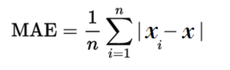
It takes mod of the difference and finds the average of errors across the dataset.

Binary Classification Loss Functions:

A binary classification problem mean that our target variable has only two types of value for e.g. 0 & 1 or -1 & 1. This mean that the output variable only has two classes and the loss is to be calculated accordingly.

• Binary Cross-Entropy Loss:

Popularly known as log loss, the loss function outputs a probability for the predicted class lying between 0 and 1. The formula shows how binary cross-entropy is calculated.

This loss function is considered by default for most of the binary classification problems. Looking at the formula, one question that comes to mind is, “Why do we need log?”. The loss functions should be able to penalize wrong prediction which is done with the help of negative log. If the prediction is correct and the probability is 1, the value will be zero which is ideal, but if it is lesser than zero then the number becomes negative. To simplify the interpretation of the penalty we use the negative sign with log to make the error positive. The above formula will be valid if the number of classes are 2. If you want to extend this logic to more than 2 classes, then simply calculate the probability for each class label per observation and sum the result.

• Hinge Loss

Hinge loss was originally developed for SVM. The simple intuition behind hinge loss is, it works on the difference of sign. For e.g. the target variable has values like -1 and 1 and the model predicts 1 whereas the actual class is -1, the function will impose a higher penalty at this point because it can sense the difference in the sign. The below given formula would work if the class labels are -1 and +1.

• Squared Hinge Loss:

Squared hinge loss is nothing but an extension to hinge loss. At times we don’t need to know the probabilities of how certain the classifier is about the output. Suppose the problem requires an output which will either be yes or no, then you could use squared hinge loss to deal with it. The below formula would work if the class labels are -1 and +1.

Multiclass Classification Loss Functions:

Multiclass classifications loss functions would be used for a problem involving more than two classes. For e.g. if we are trying to classify cuisines based on different ingredients required for the preparation, types of cuisines would become the class labels.

• Mutli-class cross entropy:

For multi-class cross entropy, it would be better if the target is a one-hot encoded vector. 

Here p(x) is the actual probability of the class and q(x) is the predicted probability. Perform this calculation for all the classes and sum them. This will give you the value of your loss function. 

• Sparse Multi-Class Loss Function:

As aforementioned, for mutli-class cross entropy we need the target variable to be in one-hot encoded form. At times this could be a problem when we have many classes. To solve this problem, we could use sparse mutli-class classification. This loss function doesn’t need the target variable to be one-hot encoded. One could consider this as an extension to the Multi-Class Cross Entropy loss function and can be implemented in less than a line of code.

• Kullback Leibler Divergence Loss:

KL Divergence Loss is used for complex problems. Here the loss function compares the distribution of the actual and the predicted values. If they are the same then the loss function is 0 and if they are not, the value of the loss function increases gradually as the distribution deviates from the original distribution.