The Approximate Nearest Neighbour (A-NN) search algorithm returns points that are closest to the query point and whose distance from the query point is a maximum of a fixed amount of times from the query to its nearest points. The algorithm captures the approximate distance between the query point and its nearest neighbours. A-NNs can solve multi-class classification tasks. In this article, we will be using A-NNoy to demonstrate the A-NN algorithm. Following are the topics to be covered.

Table of contents

1. What is the Nearest Neighbour search?
2. What is the Approximate Nearest Neighbour?
3. About ANNoy
4. Demonstrating A-NN using ANNoy

Let’s start with understanding the approximate nearest neighbour.

What is the Nearest Neighbour search?

Nearest neighbour search is a basic tool for information retrieval. The task is to find the most similar items encountered in the past when a new data item is provided. As such they help place the new item in context, for example, determining whether it is something familiar that can be handled easily or something novel that requires special attention. In particular, the nearest neighbours can be used to predict an outcome for the new instance with prior knowledge of the labels.

The algorithmic problem 

If given a sample, the nearest neighbour (NN) of a query is the point in the sample that is closest to the query point under some distance function of interest. Finding the nearest neighbour naively takes a certain amount of time, which can be a serious deterrent in many practical settings with larger samples. To speed this up, can a data structure be built from the sample that will permit subsequent queries to be answered quickly? 

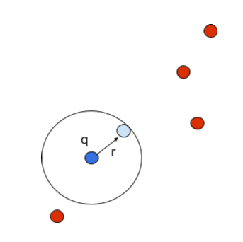
(Nearest Neighbour)

In the above representation, the q is the query point and the nearest data point is calculated and classified under the label, r is the distance. For one-dimensional data, the solution is simple: a sorted version of the sample can be used to find the nearest neighbour of any query in less than half the time with a binary search. But extending this to higher dimensions is more difficult. 

A particularly tricky case is when the data points in the sample and query are all picked at random from the surface of the unit sphere in multidimensional space. This is also known as the curse of dimensionality. So, to mitigate this curse Approximate Nearest neighbour was developed.

Why is high dimensional data a problem?

Observation becomes harder to cluster when there are too many features in the dataset, this causes every observation in the dataset to appear equally distant from all the others. As clustering uses a distance measure such as Euclidean distance to quantify the similarity between observations, it becomes impossible to find a model that can describe the relationship between the predictor variables and the response variable. 

Are you looking for a complete repository of Python libraries used in data science, check out here.

What is the Approximate Nearest Neighbour?

In the approximate nearest neighbour, we take an approximate distance from the query point and classify the data point under the query. As in the representation below, we can observe that the algorithm is considering another data point other than the point which is ‘r’ distant from the query and for calculating the distance it’s considering an approximate distance ‘cr’.

Mathematically we can state it as, given a sample with data points, let’s assume those points to be P which is present in a metric space. We need to build a data structure that, given any query point such that the point in the metric space contains a point in P, and the sample returns any point in metric dimensional space. 

(Approximate Nearest Neighbour)

If we compare both the figures we can easily observe the difference that the A-NN algorithm considered two data points to be the nearest neighbours since it took an approximate distance from the query. This technique could seem to be wrong because it does not take the absolute distance just like K- nearest neighbours do but to detail with high dimensional data taking an absolute distance could be a risky task for the algorithm. Since in high dimensional data the number of observations is lesser than the number of features which will result in missed calculations and the model will be overfitting. 

• Overfitting occurs when a function is too closely aligned to a limited set of data points. So, the model fails to capture all the data points in the dimensional space. A low bias and high variance in the data model tend to be overfit.

But this raises the question if A-NN is that good then why do we even use K-nearest neighbour (KNN).

Difference between KNN and A-NN

In the prediction phase of KNN, all training points are searched for k-nearest neighbours, whereas in A-NN this search is only carried out on a subset of training candidate points.

About ANNoy

ANNOY (Approximate Nearest Neighbors Oh Yeah) is a library that searches for points in space that are close to a query point. It has the ability to use static files as indexes which means a large data structure is mapped into memory so that many processes can access the same data.  

A-NNoy separates index creation from index loading, so the user can easily pass around indexes as files and load them into memory quickly. A-NNoy also tries to minimise memory footprint so the indexes themselves are quite small. It supports very high dimensional but very sparse datasets. A sparse dataset has the advantage that only the non-zero features of every instance need to be stored.

Demonstrating A-NN using ANNoy

In this article, we will be using a Word2Vec model to categorise words with the help of the Approximate Nearest neighbour algorithm. The A-NN algorithm will be implemented by using ANNoy.

Install A-NNoy:

! pip install annoy

Importing some necessary libraries.

import gensim, os
from gensim.models.word2vec import Word2Vec
from gensim.similarities.index import AnnoyIndexer
import matplotlib.pyplot as plt, time

Build the word2vec model:

test_data_dir = '{}'.format(os.sep).join([gensim.__path__[0], 'test', 'test_data']) + os.sep
lee_train_file = test_data_dir + 'lee_background.cor'
 
class MyText(object):
    def __iter__(self):
        for line in open(lee_train_file):
            yield line.lower().split()
 
sentences = MyText()
                
model = Word2Vec(sentences, min_count=1)
 
print(model)

Creating indexer:

An indexer is needed to be created in order to use ANNoy in gensim. This will create indexes based on the trees in the model so that they could be referred to. 

annoy_index = AnnoyIndexer(model,100)

The model is trained, and the indexer is set. Now we are ready to make a query, let’s find the top 5 most similar words to “army” in the lee corpus. To make a similarity query we will use Word2Vec.most_similar with an added parameter, indexer.

vector = model["army"]
approximate_neighbors = model.most_similar([vector], topn=5, indexer=annoy_index)
for neighbor in approximate_neighbors:
    print(neighbor)

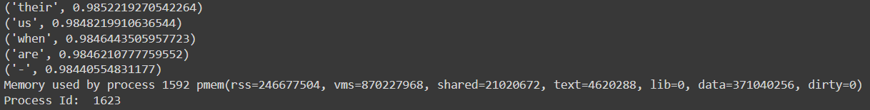
These are the top 5 similar words related to “army”. We can accept these since the closer the cosine similarity of a vector is to 1, the more similar that word is to the query.

Let’s see how ANNoy saves memory and processes faster than any other A-NN algorithm.

%%time
 
from gensim import models
from gensim.similarities.index import AnnoyIndexer
from multiprocessing import Process
import os
import psutil
 
model.save('/tmp/mymodel')
 
def f(process_id):
    print ('Process Id: ', os.getpid())
    process = psutil.Process(os.getpid())
    new_model = models.Word2Vec.load('/tmp/mymodel')
    vector = new_model["army"]
    annoy_index = AnnoyIndexer()
    annoy_index.load('index')
    annoy_index.model = new_model
    approximate_neighbors = new_model.most_similar([vector], topn=5, indexer=annoy_index)
    for neighbour in approximate_neighbors:
        print (neighbour)
    print ('Memory used by process '+str(os.getpid()), process.memory_info())
 
p1 = Process(target=f, args=('1',))
p1.start()
p1.join()
p2 = Process(target=f, args=('2',))
p2.start()
p2.join()

Here the indexes are shared between two processes by memory mapping. This method uses less total RAM as it is shared.

Let’s have a look at variations in timing and performance of the model according to the number of trees.

Plotting variation in initialization time:

import matplotlib.pyplot as plt, time
x_cor = []
y_cor = []
for x in range(100):
    start_time = time.time()
    AnnoyIndexer(model, x)
    y_cor.append(time.time()-start_time)
    x_cor.append(x)
 
plt.plot(x_cor, y_cor)
plt.title("Variation in initalization time w.r.t number of trees")
plt.ylabel("Initialization time (s)")
plt.xlabel("num_tress")
plt.show()

The initialization time of the ANNoy indexer varies in a linear relationship which is as the number of trees increases the initialization time increases. But we could observe a high variation between 40 to 50 and 80 to 90 this may be because of less core availed at that time of initialization because the ‘most_similar’ method is using numpy operations in the form of the dot product to find the similars so needs a more number of cores to process the calculations.

Plotting variation in initialization time:

exact_results = [element[0] for element in model.most_similar([model.wv.syn0norm[0]], topn=100)]
x_axis = []
y_axis = []
for x in range(1,80):
    annoy_index = AnnoyIndexer(model, x)
    approximate_results = model.most_similar([model.wv.syn0norm[0]],topn=100, indexer=annoy_index)
    top_words = [result[0] for result in approximate_results]
    x_axis.append(x)
    y_axis.append(len(set(top_words).intersection(exact_results)))
    
plt.plot(x_axis, y_axis)
plt.title("Variation in performance")
plt.ylabel("% accuracy")
plt.xlabel("num_trees")
plt.show()

The accuracy increases as the number of trees increases (linear) but the higher number of trees could result in overfitting so an optimal number of trees should be selected with an optimal accuracy score.

Final verdict

An approximate nearest neighbour algorithm (A-NN) is perfect for high-dimensional data, since the more dimensions there are, the more the algorithm’s runtime is determined by the number of dimensions, instead of the number of input instances as usually assumed. Many times we do not need an accurate answer but an optimal answer which could be obtained easily and faster.

References

• Link to the above code
• Genism with A-NNoy