Choosing features is an important step in constructing powerful machine learning models. The difficulty of picking input variables that are useful for predicting a target value for each occurrence in a dataset is referred to as feature selection. This article focuses on the feature selection wrapper method using the Shapley values. This method would be implemented using the Powershap python library. Following are the topics to be covered.

Table of contents

1. Description of Shapley value
2. How Shapley value would be used for feature selection?
   1. The explain component 
   2. The core component
3. Implementing feature selection with Powershap

The weighted average of marginal contributions is the Shapley value. The technique tries to explain why an ML model returns the results it does on the given input. Let’s deep dive into Shapley values.

Description of Shapley value

The Shapley value is a game theory solution notion that entails equitably sharing both profits and costs to numerous agents operating in the coalition. When two or more players or components are involved in a strategy to obtain a desired outcome or payout, this is referred to as a game theory. 

The Shapley value is most applicable when the contributions of each actor are uneven, yet each person works together to achieve the gain or payout. The Shapley value assures that each actor receives the same or more than they would if they were operating separately. The value obtained is crucial since there is no motivation for actors to interact otherwise.

For example, for a model determining whether an application should be granted a credit card, we would want to know why a retiree (say, person A) has been rejected a credit card application, or why the model estimates the likelihood of default is 80%.

Here there is a need for a reason behind the rejection of person A while others are not, or why that individual is thought to have an 80% likelihood of default when the typical applicant obtains just a 20% chance from the model. 

When comparing all approved candidates, it is discovered that the common reasons for rejection, such as individual A’s need to significantly improve their salary. However, by comparing individual A to all other accepted retired candidates, individuals may discover that the expected high default rate is due to above-average debt. Shapley values are contextualized using comparison groups in this way.

As a result, the Shapley value technique takes the model output on the individual as well as some comparison group of applicants and attributes how much of the difference between the person and the comparison group is accounted for by each characteristic. For example, there is a 70% gap to explain between an 80% forecasted default rate and a 10% expected default rate for accepted retiree applicants. Shapley may allocate 50% of an individual’s loan debt, 15% to low net worth, and 5% to low income in retirement, based on the average marginal contribution of each characteristic to the total score difference.

Are you looking for a complete repository of Python libraries used in data science, check out here.

How Shapley value would be used for feature selection?

The technique is based on the assumption that a known random characteristic should have a lesser influence on predictions than an informative feature. The algorithm is made up of two parts that work together to achieve feature selection.

The Explain component

A single known random uniform (RandomUniform) feature is introduced to the feature set for training a machine learning model in the Explain component. Using the Shapley values on an out-of-sample subset of the data allows you to quantify the influence of each feature on the outcome. To determine the real unbiased influence, the Shapley values are tested on unseen data. Finally, the absolute value of all Shapley values is calculated and averaged to get the overall average influence of each feature. A single mean value is employed here, making statistical comparisons easy.

Furthermore, when using absolute Shapley values, both positive and negative values are included in the overall effect, which may result in a different distribution than the Gini significance. This procedure is then repeated several times, with each iteration retraining the model with a different random feature and using a different subset of the data to quantify the Shapley values, resulting in an empirical distribution of average impacts that will be used for the statistical comparison.

The Core component

Given the average impact of each feature for each iteration, the influence of the random feature in the core powershap component can be compared. The percentile formula is used to quantify this comparison, which consists of an array of average Shapley values for a single feature with the same length as the number of repetitions, a single value, and the indicator function. This formula computes the proportion of iterations in which a single value was greater than the iteration’s average shap-value and may thus be regarded as the p-value. The formula produces p-values that are lower than what should be seen. Smaller p-values are more prevalent as the number of iterations is reduced.

Since the hypothesis indicates that the impact of the random feature should be smaller on average than the impact of any informative feature, all impacts of the random feature are averaged again, yielding a single value that can be utilized in the percentile function. This yields a p-value for each unique characteristic. This p-value shows the proportion of situations in which the characteristic is less essential than a random feature on average. A heuristic implementation of a one-sample one-tailed student-t smaller statistic test may be performed using the hypothesis and these p-value estimates. 

• Null hypothesis (H0): The random feature is not more important than the tested feature. 
• Alternative hypothesis (H1): The random feature is more important than the tested feature.

As a result, in this statistical test, the positive class indicates a correct null hypothesis. In contrast to a normal student-t statistic test, which assumes a typical Gaussian distribution, this heuristic approach does not presume a distribution on the tested feature affects scores. The collection of informative characteristics may then be found and output is given a threshold p-value.

Implementing feature selection with Powershap

This article uses a dataset related to the classification of safe drinking water based on different features like ph-value, hardness, TDS, etc. For detailed knowledge of the features read here. 

Powershap is a wrapper-based feature selection approach that employs statistical hypothesis testing and power calculations on Shapley values to enable rapid and straightforward feature selection.

Let’s start by installing the Powershap package.

! pip install powershap

Import necessary libraries

import pandas as pd
from powershap import PowerShap
 
from sklearn.model_selection import train_test_split
from sklearn.linear_model import LogisticRegressionCV
from sklearn.ensemble import GradientBoostingClassifier

Reading data and preprocessing

data=pd.read_csv('water_potability.csv')
data[:5]

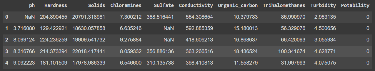
data_utils=data.dropna(axis=0)
X=data_utils.drop(['Potability'],axis=1)
y=data_utils['Potability']

Splitting the data into standard 30:70 ratio test and train respectively.

X_train, X_test, y_train, y_test = train_test_split(X, y, test_size=0.30, shuffle=True, random_state=42)

Build the Powershap function by defining the models to be used for the classification. Currently only sklearn is supported with the Powershap package. For this article, we are building two selectors one with Gradient Boosting Classifier algorithm and the other with Logistic Regression CV algorithm

selector = PowerShap(
    model = GradientBoostingClassifier(),
    automatic=True, limit_automatic=100)
selector.fit(X_train, y_train)

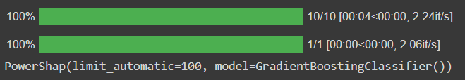
selector.transform(X_test)

This will give the features with high impact values and with a true null hypothesis that the given feature is more important than the random feature.

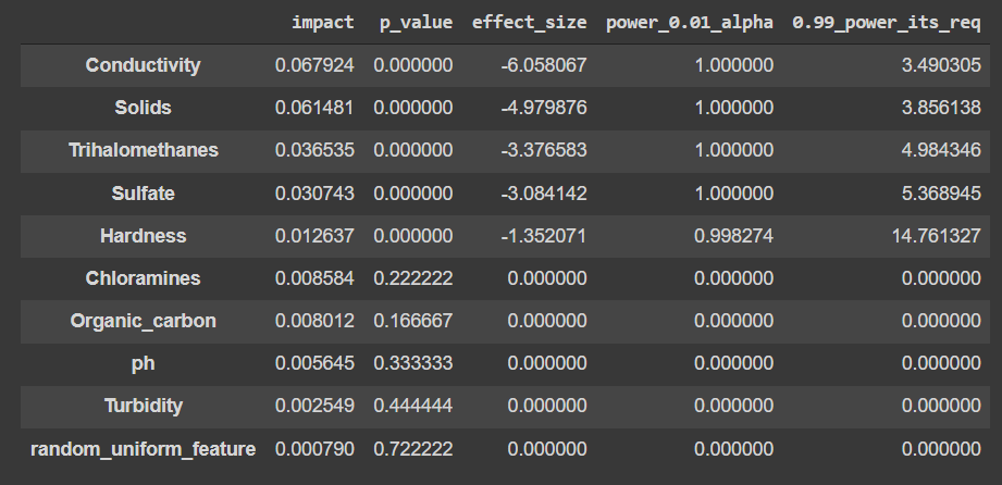
According to the algorithm, there are three important features out of 10 while using the Gradient Boosting Classifier base model. We can also see the impact score and other statistical values by using this code.

selector._processed_shaps_df

Similarly checking for the other selector.

selector_2 = PowerShap(
    model = LogisticRegressionCV(max_iter=200),
    automatic=True, limit_automatic=100,
)
selector_2.fit(X_train, y_train)

selector_2.transform(X_test)

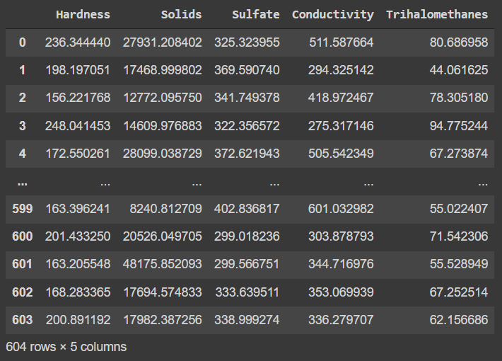
According to the algorithm, there are five important features out of 10 while using the Logistic regression CV for 200 iterations.

selector_2._processed_shaps_df

Conclusion

The Shapley values and statistical tests for a wrapper feature selection approach were used to determine the relevance of features, and the findings were significant. To achieve rapid, strong, and reliable feature selection, the powershap performs power calculations to optimise the number of needed iterations in an automated mode. With this article, we have understood the usage of Shapley values for feature selection and implementation with Powershap.

References

• Link to the above code
• Read more about Shapley value