Today, with the advancement in technology, Survival analysis is frequently used in the pharmaceutical sector. It analyses a given dataset in a characterised time length before another event happens. The Kaplan Meier estimator is an estimator used in survival analysis by using the lifetime data. In medical research, it is frequently used to gauge the part of patients living for a specific measure of time after treatment.

Here, we will implement the survival analysis using the Kaplan Meier Estimate to predict whether or not the patient will survive for at least one year.

About the dataset

The dataset can be downloaded from the following link. It gives the details of the patient’s heart attack and condition.

Code Implementation

Install all the libraries required for this project.

pip install lifelines
import pandas as pd
import numpy as np
import matplotlib.pyplot as plt
import seaborn as sns
import statistics
from sklearn.impute import SimpleImputer
from lifelines import KaplanMeierFitter, CoxPHFitter
from lifelines.statistics import logrank_test
from scipy import stats

Reading the Data

df = pd.read_csv("echocardiogram.csv")
df.head()

Data Pre-Processing

Let us check for missing values and impute them with mean values.

mean = SimpleImputer(missing_values = np.nan, strategy = 'mean')
Columns = ['age', 'pericardialeffusion', 'fractionalshortening', 'epss', 'lvdd', 'wallmotion-score']
X = mean.fit_transform(df[Columns])
df_X = pd.DataFrame(X,
                    columns = Columns)
keep = ['survival', 'alive']
df_keepcolumn = df[keep]
df = pd.concat([df_keepcolumn, df_X], axis = 1)
df = df.dropna() 
print(df.isnull().sum())
print(df.shape)

Create a new column  

df.loc[df.alive == 1, 'dead'] = 0
df.loc[df.alive == 0, 'dead'] = 1
df.groupby('dead').count()

Kaplan Meier Curve

kmf = KaplanMeierFitter()
X= df['survival']
Y = df['dead']
kmf.fit(X, event_observed = Y)
kmf.plot()
plt.title("Kaplan Meier estimates")
plt.xlabel("Month after heart attack")
plt.ylabel("Survival")
plt.show()

From the plot we can see that the survival rate decreases with the increase in the number of months.The Kaplan estimate is 1 for the initial days following the heart treatment.It gradually decreases to around 0.05 after 50 months.

print("The median survival time :",kmf.median_survival_time_)

The average survival time of patients is 29 months.Given below is the KM_estimate that gives the probability of survival after the treatment.

print(kmf.survival_function_)

age_group = df['age'] < statistics.median(df['age'])
ax = plt.subplot(111)
kmf.fit(X[age_group], event_observed = Y[age_group], label = 'below 62')
kmf.plot(ax = ax)
kmf.fit(X[~age_group], event_observed = Y[~age_group], label = 'above 62')
kmf.plot(ax = ax)
plt.title("Kaplan Meier estimates by age group")
plt.xlabel("Month after heart attack")
plt.ylabel("Survival")

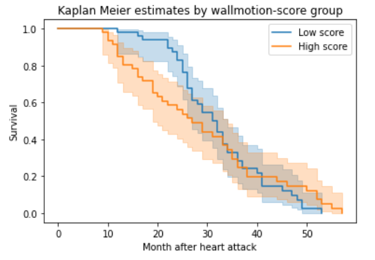
Kaplan Meier Curve Using Wallmotion Score

As we can see that the difference between the age groups is less in the previous step, it is good to analyse our data using the wallmotion-score group.The Kaplan estimate for age group below 62 is higher for 24 months after the heart condition. After it, the survival rate is similar to the age group above 62.

score_group = df['wallmotion-score'] < statistics.median(df['wallmotion-score'])
ax = plt.subplot(111)
kmf.fit(X[score_group], event_observed = Y[score_group], label = 'Low score')
kmf.plot(ax = ax)
kmf.fit(X[~score_group], event_observed = Y[~score_group], label = 'High score')
kmf.plot(ax = ax)
plt.title("Kaplan Meier estimates by wallmotion-score group")
plt.xlabel("Month after heart attack")
plt.ylabel("Survival")

Conclusion

In this article, we have discussed the survival analysis using the Kaplan Meier Estimate. It also helps us to determine distributions given the Kaplan survival plots. Further, we researched on the survival rate of different age groups after following the heart treatment. Finally, it is advisable to look into survival analysis in detail.