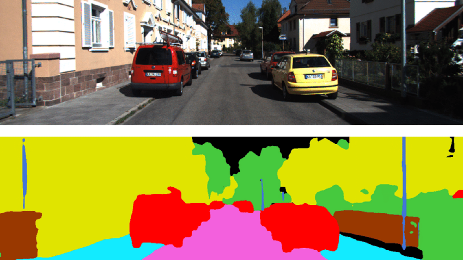
Semantic Segmentation laid down the fundamental path to advanced Computer Vision tasks such as object detection, shape recognition, autonomous driving, robotics, and virtual reality. Semantic segmentation can be defined as the process of pixel-level image classification into two or more Object classes. It differs from image classification entirely, as the latter performs image-level classification. For instance, consider an image that consists mainly of a zebra, surrounded by grass fields, a tree and a flying bird. Image classification tells us that the image belongs to the ‘zebra’ class. It can not tell where the zebra is or what its size or pose is. But, semantic segmentation of that image may tell that there is a zebra, grass field, a bird and a tree in the given image (classifies parts of an image into separate classes). And it tells us which pixels in the image belong to which class.
In this article, we discuss semantic segmentation using TensorFlow Keras. Readers are expected to have a fundamental knowledge of deep learning, image classification and transfer learning. Nevertheless, the following articles might fulfil these prerequisites with a quick and clear understanding:
- Getting Started With Deep Learning Using TensorFlow Keras
- Getting Started With Computer Vision Using TensorFlow Keras
- Exploring Transfer Learning Using TensorFlow Keras
Let’s dive deeper into hands-on learning.
Create the Environment
Import necessary frameworks, libraries and modules.
 import numpy as np
 import tensorflow as tf
 from tensorflow import keras
 import cv2
 from scipy import io
 import tensorflow_datasets as tfds
 import matplotlib.pyplot as plt
Prepare Segmentation Dataset
We use Clothing Co-Parsing public dataset as our supervised dataset. This dataset has 1000 images of people (one person per image). There are 1000 label images corresponding to those original images. Label images have 59 segmented classes corresponding to classes such as hair, shirt, shoes, skin, sunglasses and cap.
Download the images from the source.
!git clone https://github.com/bearpaw/clothing-co-parsing.git
Output:
Have a look at the dataset source files.
!ls clothing-co-parsing/
Output:
Input images are in the photos directory, and labelled images are in the annotations directory. Let’s extract the input images from the respective source directory.
 images = []
 for i in range(1,1001):
     url = './clothing-co-parsing/photos/%04d.jpg'%(i)
     img = cv2.imread(url)
     img = cv2.cvtColor(img, cv2.COLOR_BGR2RGB)
     images.append(tf.convert_to_tensor(img))
Let’s extract the labelled images (segmented images) from the respective source directory.
 masks = []
 for i in range(1,1001):
     url = './clothing-co-parsing/annotations/pixel-level/%04d.mat'%(i)
     file = io.loadmat(url)
     mask = tf.convert_to_tensor(file['groundtruth'])
     masks.append(mask)
How many examples do we have now?
len(images), len(masks)
Output:
As mentioned in the source files, there are 1000 images and 1000 labels. Visualize some images to get better insights.
 plt.figure(figsize=(10,4))
 for i in range(1,4):
     plt.subplot(1,3,i)
     img = images[i]
     plt.imshow(img, cmap='jet')
     plt.colorbar()
     plt.axis('off')
 plt.show()
Output:
The images are 3-channel colour images with values ranging from 0 to 255. Images seem to have different sizes. We need to scale images and resize them to some common shape. Let’s visualize label images corresponding to the above input images.
 plt.figure(figsize=(10,4))
 for i in range(1,4):
     plt.subplot(1,3,i)
     img = masks[i]
     plt.imshow(img, cmap='jet')
     plt.colorbar()
     plt.axis('off')
 plt.show()
Output:
Each colour in the above images refer to a specific class. We observe that the person and her/his wearings are segmented, leaving the surrounding unsegmented.
masks[0].numpy().min(), masks[0].numpy().max()
Output:
The label values start at 0 and go all the way through 59.
Model Selection
We enter into deep learning now. We have to build a computer vision model that can convert an input image into a segmented image (also called masked image or label image). Building a model from scratch and training it is not a good idea as we have very limited data for training (1000 images are insufficient for 59 unbalanced classes). So we prefer a pre-trained model through transfer learning.
By understanding how semantic segmentation works, we can easily come up with an idea of how to choose our pre-trained model. One of the popular architectural approaches is FCNN (Fully Convolutional Neural Networks). In contrast to CNNs in image classification, where the decision head is made up of dense layers, an FCNN is made up of layers related to convolutional operations only. Because the final output is an image of a shape identical to the input image.
An FCNN contains two parts: an encoder and a decoder. An encoder is a downstack of convolutional neural layers that extract features from the input image. A decoder is an upstack of transpose convolutional neural layers that builds the segmented image from the extracted features. The sizes of feature maps go down while downsampling (e.g. 128, 64, 32, 16, 8, 4 – in order), and they go up while upsampling (e.g. 4, 8, 16, 32, 64, 128 – in order).
Among FCNNs, U-Net is one of the successful architectures acclaimed for its performance in Medical Image Segmentation. It encourages skip connections between a few specific-sized layers of downstack and upstack. Skip-connections yield better performance because of the truth that upstack struggles to build finer details of the image on its own during upsampling. Skip-connections bye-pass a large stack of layers to feed finer details from a downstack layer to its corresponding upstack layer.
Original U-Net architecture for Medical Image Segmentation (source)
Here, we wish to use the functional approach of U-Net architecture, but we will have our own architecture suitable to our task. The downstack can be a pre-trained CNN, trained for image classification (e.g. MobileNetV2, ResNet, NASNet, Inception, DenseNet, or EfficientNet). It can effectively extract the features. But, we have to build our upstack to match our classes (here, 59), build skip-connections, and train it with our data.
We prefer a pre-trained DenseNet121 to be the downstack that can be obtained through transfer learning and build the upstack with pix2pix, a publicly available generative upstack template (it saves our time and code).
Build Downstack Model
Load DenseNet121 from in-built applications.
 base = keras.applications.DenseNet121(input_shape=[128,128,3],
                                       include_top=False,
                                       weights='imagenet')
Output:
len(base.layers)
Output:
The DenseNet121 model has 427 layers. We need to identify suitable layers whose output will be used for skip connections. Plot the entire model, along with the feature shapes.
keras.utils.plot_model(base, show_shapes=True)
Necessary portions from the output:
We select the final ReLU activation layer for each feature map size, i.e. 4, 8, 16, 32, and 64, required for skip-connections. Write down the names of the selected ReLU layers in a list.
 skip_names = ['conv1/relu', # size 64*64
              'pool2_relu',  # size 32*32
              'pool3_relu',  # size 16*16
              'pool4_relu',  # size 8*8
              'relu'        # size 4*4
              ]
Obtain the outputs of these layers.
 skip_outputs = [base.get_layer(name).output for name in skip_names]
 for i in range(len(skip_outputs)):
     print(skip_outputs[i])
Output:
Build the downstack with the above layers. We use the pre-trained model as such, without any fine-tuning.
 downstack = keras.Model(inputs=base.input,
                        outputs=skip_outputs)
 downstack.trainable = False
Build Upstack Model
Build the upstack using an upsampling template.
 !pip install -q git+https://github.com/tensorflow/examples.git
 from tensorflow_examples.models.pix2pix import pix2pix
 # Four upstack blocks for upsampling sizes
 # 4->8, 8->16, 16->32, 32->64
 upstack = [pix2pix.upsample(512,3),
           pix2pix.upsample(256,3),
           pix2pix.upsample(128,3),
           pix2pix.upsample(64,3)]
We can explore the individual layers in each upstack block.
upstack[0].layers
Output:
Integrate the Segmentation Model
Build a U-Net model by merging downstack and upstack with skip-connections.
 # define the input layer
 inputs = keras.layers.Input(shape=[128,128,3])
 # downsample
 down = downstack(inputs)
 out = down[-1]
 # prepare skip-connections
 skips = reversed(down[:-1])
 # choose the last layer at first 4 --> 8
 # upsample with skip-connections
 for up, skip in zip(upstack,skips):
     out = up(out)
     out = keras.layers.Concatenate()([out,skip])
 # define the final transpose conv layer
 # image 128 by 128 with 59 classes
 out = keras.layers.Conv2DTranspose(59, 3,
                                   strides=2,
                                   padding='same',
                                   )(out)
 # complete unet model
 unet = keras.Model(inputs=inputs, outputs=out)
Visualize our U-Net model.
keras.utils.plot_model(unet, show_shapes=True)
Output:
Preprocess Data
The model is perfectly ready. We can start training if data preprocessing is performed. Since we have limited images, we prepare more data through augmentation.
 def resize_image(image):
     image = tf.cast(image, tf.float32)
     # scale values to [0,1]
     image = image/255.0
     # resize image
     image = tf.image.resize(image, (128,128))
     return image
 def resize_mask(mask):
     mask = tf.expand_dims(mask, axis=-1)
     mask = tf.image.resize(mask, (128,128))
     mask = tf.cast(mask, tf.uint8)
     return mask
Resize images and masks to the size 128 by 128.
 X = [resize_image(i) for i in images]
 y = [resize_mask(m) for m in masks]
Split the data into train and validation sets.
 from sklearn.model_selection import train_test_split
 train_X, val_X,train_y, val_y = train_test_split(X,y,
                                                       test_size=0.2,
                                                       random_state=0
                                                      )
 train_X = tf.data.Dataset.from_tensor_slices(train_X)
 val_X = tf.data.Dataset.from_tensor_slices(val_X)
 train_y = tf.data.Dataset.from_tensor_slices(train_y)
 val_y = tf.data.Dataset.from_tensor_slices(val_y)
 train_X.element_spec, train_y.element_spec, val_X.element_spec, val_y.element_spec
Output:
Zip input images and ground truth masks.
 train = tf.data.Dataset.zip((train_X, train_y))
 val = tf.data.Dataset.zip((val_X, val_y))
We have 800 train examples. That’s too low for training. We define a couple of augmentation functions to generate more train examples.
 def brightness(img, mask):
     img = tf.image.adjust_brightness(img, 0.1)
     return img, mask

 def gamma(img, mask):
     img = tf.image.adjust_gamma(img, 0.1)
     return img, mask

 def hue(img, mask):
     img = tf.image.adjust_hue(img, -0.1)
     return img, mask

 def crop(img, mask):
     img = tf.image.central_crop(img, 0.7)
     img = tf.image.resize(img, (128,128))
     mask = tf.image.central_crop(mask, 0.7)
     mask = tf.image.resize(mask, (128,128))
     mask = tf.cast(mask, tf.uint8)
     return img, mask

 def flip_hori(img, mask):
     img = tf.image.flip_left_right(img)
     mask = tf.image.flip_left_right(mask)
     return img, mask

 def flip_vert(img, mask):
     img = tf.image.flip_up_down(img)
     mask = tf.image.flip_up_down(mask)
     return img, mask

 def rotate(img, mask):
     img = tf.image.rot90(img)
     mask = tf.image.rot90(mask)
     return img, mask
Apply augmentation to the data with the above functions. With 7 augmentation functions and 800 input examples, we can get 7*800 = 5600 new examples. Including original examples, we get 5600+800 = 6400 examples for training. That sounds good!
 train = tf.data.Dataset.zip((train_X, train_y))
 val = tf.data.Dataset.zip((val_X, val_y))

 # perform augmentation on train data only
 a = train.map(brightness)
 b = train.map(gamma)
 c = train.map(hue)
 d = train.map(crop)
 e = train.map(flip_hori)
 f = train.map(flip_vert)
 g = train.map(rotate)

 train = train.concatenate(a)
 train = train.concatenate(b)
 train = train.concatenate(c)
 train = train.concatenate(d)
 train = train.concatenate(e)
 train = train.concatenate(f)
 train = train.concatenate(g)
Prepare data batches. Shuffle the train data.
 BATCH = 64
 AT = tf.data.AUTOTUNE
 BUFFER = 1000
 STEPS_PER_EPOCH = 800//BATCH
 VALIDATION_STEPS = 200//BATCH
 train = train.cache().shuffle(BUFFER).batch(BATCH).repeat()
 train = train.prefetch(buffer_size=AT)
 val = val.batch(BATCH)
Train the Model
Let’s check whether everything is good with the data and the model by sampling one example image and predict it with the untrained model.
 example = next(iter(train))
 preds = unet(example[0])
 plt.imshow(example[0][60])
 plt.colorbar()
 plt.show()
Output:
 pred_mask = tf.argmax(preds, axis=-1)
 pred_mask = tf.expand_dims(pred_mask, -1)
 plt.imshow(pred_mask[0])
 plt.colorbar()
Output:
Compile the model with RMSprop optimizer, Sparse Categorical Cross-entropy loss function and accuracy metric. Train the model for 20 epochs.
 unet.compile(loss= keras.losses.SparseCategoricalCrossentropy(from_logits=True),
             optimizer=keras.optimizers.RMSprop(lr=0.001),
             metrics=['accuracy'])

 hist = unet.fit(train,
                validation_data=val,
                steps_per_epoch=STEPS_PER_EPOCH,
                validation_steps=VALIDATION_STEPS,
                epochs=50)
A portion of the output:
Performance Evaluation
Let’s check how our model performs.
 img, mask = next(iter(val))
 pred = unet.predict(img)

 plt.figure(figsize=(10,5))
 for i in pred:
     plt.subplot(121)
     i = tf.argmax(i, axis=-1)
     plt.imshow(i,cmap='jet')
     plt.axis('off')
     plt.title('Prediction')
     break

 plt.subplot(122)
 plt.imshow(mask[0], cmap='jet')
 plt.axis('off')
 plt.title('Ground Truth')
 plt.show()
Output:
We observe closeness to a certain level. By training for more epochs, we can obtain improvement in the results. Let’s plot the performance curve for accuracy.
 history = hist.history
 acc=history['accuracy']
 val_acc = history['val_accuracy']
 plt.plot(acc, '-', label='Training Accuracy')
 plt.plot(val_acc, '--', label='Validation Accuracy')
 plt.xlabel('Epochs')
 plt.ylabel('Accuracy')
 plt.legend()
 plt.show()
Output:
The amount of training data plays a vital role in performance in a deep learning model. Limited data, in our case, maybe one reason for relatively poor performance. By tuning hyperparameters carefully, improving or changing model architectures, and increasing training data, we could achieve performance improvements.
The Notebook with the above code implementation.
Wrapping Up
In this article, we have discussed semantic segmentation using TensorFlow Keras. We have explored the concepts, architecture, working principle of a semantic segmentation deep learning model with a practical dataset. Further, we have discussed some image data augmentation techniques to multiply the amount of our training data.

