Suppose you are asked to prove how useful a feature could be. Let’s say you have to estimate the number of users on your platform that would benefit from a certain feature or change on your product.

You pick a “random uniform sample” of 1% of the users. They are now exposed to the feature. In a week’s time, you have figured that 1000 users are actively using the feature.

Now the time comes for you to get the feature to be rolled out to the entire traffic. You now have to answer the question from the management on how many users could potentially benefit from this feature.

And you are going to say 100,000 because on a 1% random uniform sample, 1000 liked it. Sounds reasonable?

I am going to stop right here and ask this flip question.

Suppose there were really 100,000 people who would like this feature and benefit from it. What is the chance (or probability) that you would get this number of 1000 from this 1% sample?

I think this is where people tend to get a lot confused. I have heard answers saying that they are 100% sure. And the reasoning would be that this was a perfectly random sample, or random uniform sample, to be precise!

You can take a pause from reading this article further and see if the above makes sense and spot the fallacy here.

The way to approach this problem is the following: We need to find the following conditional probability

P(n=1000|N=100000)

where n=number of people interested in this 1% sample and N= number of people interested overall.

P(n|N) is actually a binomial distribution. Lets see how.

Chance of a interested user falling in this sample is (1 / 100) or the sample percentage s, given it is a random uniform distribution. This turns out to be the following formula:

Substituting values of n = 1000 and N = 100000 and s = 0.01, we get

In other words, the expected value of 1000 has a chance of just 1.2%

Also just to recollect, the mean of the binomial distribution is:

So the expected value is indeed 1000, but it has a pretty low probability!

I think this is an important thing to understand. I know it looks like doing a test on 1% random traffic sample does not make much sense. Let us continue to explore and see!

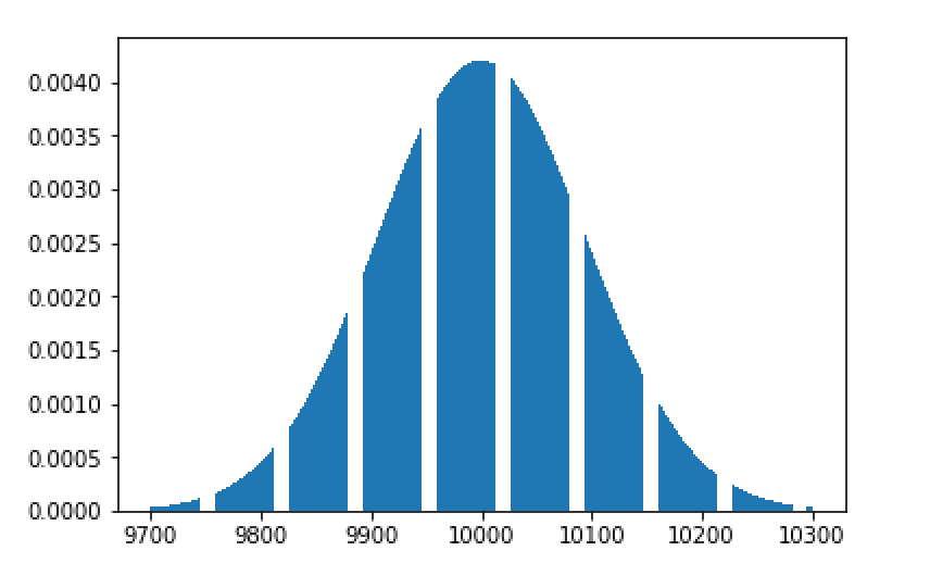
Let us, therefore, try to increase the sample size to 10%. The expected value would be 10,000. Let us compute the probability of the same.

In other words, the probability has gone down to 0.4% despite the larger sample size.

On the other hand, let us try a very very small sample size of 0.01% instead.

The probability of getting the “expected value” of 10 has now gone up close to 12.5%.

As we would all expect, the higher the sample size, we should be able to get to the true value with a higher probability, but the reverse seems to be happening. What is the fallacy here?

At this point, it is important to look not only at the individual probability but the spread of probabilities.

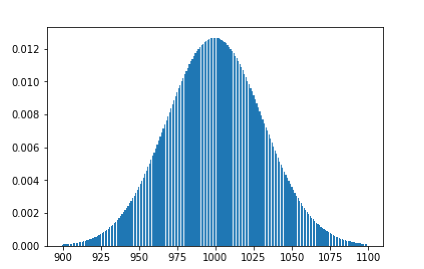
This shows that values of “n” are going to range mostly between 900 to 1100. Suppose we get n to be 1050, our estimate of N = 1050 * 100 = 105,000 instead of 100,000. This is a 5% error which one may consider to be not way of the mark.

As can now be seen from the above distribution plot, if the sampled ’n’ turns out to be 5, then the estimate for N would 50,000 — that is a 50% error!

That turns us to an important statistic we have not talked about so far — variance. Let us look at the variance at the different sample sizes.

Let us look at the standard deviation for different values of s.

The standard deviation reduces drastically as the sample size increases. Even at a sample size 1%, the standard deviation is just 3% of the mean.

How does this standard deviation help in giving me confidence that the errors are manageable? Let me introduce a concept called Chebychev inequality. Dont get overwhelmed by the formula — will explain it in a second.

This just means that the chance of a value lying k standard deviations away from mean is less than (1 / k²)!

Applying Chebychev inequality, we know that the probability of a value lying atleast 3 standard deviations away from mean is 1/(3*3) is less than 1/9 or roughly 10%.

So in our specific example, if you select a sampling rate of 1%, you can be at least 90% sure that the value you get is not more than 10% away from the mean!

I think a 90% confidence of not being more than 10% away from the mark should be sufficient for practical purposes!

PS: For the more observant, there is an inherent assumption being made that we know N prior to this. It is a slightly more advanced topic, but suffices to say that as long as N is somewhat large, say more than 5000, a 1% sampling rate should be great. This indicates that some sort of prior knowledge of N may be required — at least the range where N falls.

To recapitulate, the lessons are:

• a) The value collected from the sample is *not* going to be exact measure that you want and will have deviations from the exact measure. It is important to understand how much deviations or error from the exact measure exists.
• b) Choosing larger sample sizes minimize the chances of deviation. A 1% sampling rate is more than sufficient in most of the cases.