Titanic disaster is one of the most infamous shipwrecks in the history. During her maiden voyage en route to New York City from England, she sank killing 1500 passengers and crew on board. Various information about the passengers was summed up to form a database, which is available as a dataset at Kaggle platform. In this interesting use case, we have used this dataset to predict if people survived the Titanic Disaster or not. Parameters such as sex, age, ticket, passenger class etc. are used to train the data and used in the algorithms to predict the test data.

Different machine learning algorithms were used to train and test the model, which are listed here.

An Artificial Neural Network with two hidden layers was also used to compare the results, accuracy and time taken for both training and testing the data. The output is extracted in Binary format i.e 1s(survived) and 0s(deceased).

The input features used are as follows:

• PassengerID – This is an Unique ID given to every passenger.
• Survived – 0 for deceased and 1 for survived
• Pclass – Passenger class ranging from 1 to 3
• Name – Passenger full name with honorifics
• Sex – Male or female
• Age – Age of the passenger
• SibSp – number of siblings or spouses on board related to the specific passenger
• Parch – number of parents or children on board related to the specific passenger
• Ticket – Ticket number
• Fare – Ticket fare
• Cabin – Cabin alloted to the passenger
• Embarked – Port of embarkation (C = Cherbourg; Q = Queenstown; S = Southampton)

The above features are called as X and the feature Y is expressed as Survived(1) or Deceased(0).

Data Analysis:

There will be an instance where some of the features will not account for the classification in the final result. In this situation, we need to start analyzing all the features with respect to the target. Example: Draw a graph of Age vs Survived, Sex vs Survived, Passenger class vs Survived. We draw a graph of these, lets say its a bar graph like the picture below,

Here the Man, Woman and Child are calculated by the Sex and Age features. From the graph we can see that the woman show a high rate of survival. So this is a feature which needs to be considered.

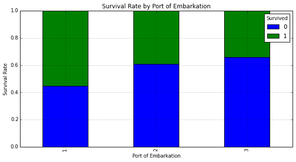
In the above graph, the port of embarkation accounts very less for the passenger’s survival, because the probability that the passenger has survived or not is around 0.5(50%) which does not hold any strong information for the prediction. So these type of features can be dropped while training the model.

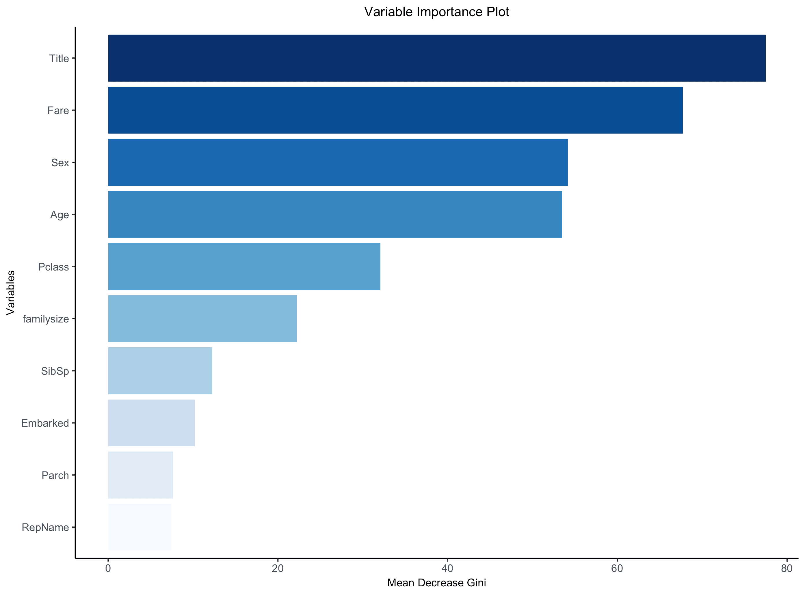
You can also consider a single category for a feature which accounts for the target class, like one among the cabins. Below is the feature importance graph showing weight-age distribution and comparison.

Data Processing:

Every data set you come across will contain NULL values or missing values. The above data frame contains NULLs in the Cabin feature. The missing values will lead to misleading results when predicting because these values have no weight-age. There are 3 approaches in which you can solve this problem.

First, you can drop or delete all the rows which has missing data to free your dataframe from the NULLs. Second, you can move them to a new category by assigning ‘U’ or unknown. Third, you can train the data which are free from the missing values from the first step and using regression technique to predict these missing values.

There are two kinds of features in this dataset. One is Continuous and the other is Categorical features. Features like Age and Fare are termed as continuous (mostly numerical values) and cabin, sex, embarked etc. are termed as categorical because it has different categories  like male and female.

In this comparison, the NULLs were assigned with the unknown for categorical data and mean of the particular continuous feature was assigned to the NULLs in continuous data.

These categorical features must be converted into sets of binary. The methods used are One Hot Encoding where each category is converted into different feature and the other is the label encoder which assigns values to each type of category. Here is the example,

One Hot Encoding: Each type of category is converted into a new feature with 0 for absent and 1 for present.

One hot encoding was used to convert the data from categorical to numerical.

Once the data analysis and data processing is done, we can move on to the application of the algorithms.

Random Forest Algorithm:

In classification, inputs are divided into two or more classes, and the learner must produce a model that assigns unseen inputs to one or more (multi-label classification) of these classes. This is typically tackled in a supervised way. Spam filtering is an example of classification, where the inputs are email (or other) messages and the classes are “spam” and “not spam”. In this model, the target classes are ‘Survived’ and ‘Deceased’

The algorithm used to train the model is Random Forest, its a non linear ensemble learning binary classifier which neglects the correlation of the data. Random forest is an advance version of decision tree. Random forests are a way of averaging multiple deep decision trees, trained on different parts of the same training set, with the goal of reducing the variance. This comes at the expense of a small increase in the bias and some loss of interpret ability, but generally greatly boosts the performance in the final model. Random forest works on the principle of Bootstrap aggregating https://en.wikipedia.org/wiki/Bootstrap_aggregating

Below is a visual understanding of how a random forest algorithm looks on the inside.

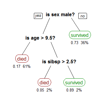
The above diagram shows how the decision trees are formed using the training data. The information gain is calculated from the entropy or gini(proportion of the target values). And using the gini coefficient the threshold is calculated, which classifies the data based on the constraint.

This model contains 3 decision trees. Here the feature Sex provides the highest information gain hence it has been allotted the decision maker in the first tree. Each passenger data is passed through these trees and based on their allocation, their survival is predicted. This model takes training data to train the model and its accuracy is tested on the test data. The data sets can be accessed here https://www.kaggle.com/c/titanic/data.

Drawbacks of Random Forest:

The algorithm used was random forest which requires very less tuning compared to algorithms like SVMs. The time taken to process the training set of data is comparatively small with an accuracy of 61% with 100 trees. Random forest is a non linear classifier which works well when there is a large amount of data in the data set. Training of these models will take time but the accuracy will also increase. The problem I faced during the training of random forest is over-fitting of the training data. Since the data is small with 891 rows, it will over-fit and give an accuracy above 90% with the training data. Even if a regularizer is used to cure the over-fitting, this account of almost 2-5% of the data when the data is already that small.  

Artificial Neural Network:

We implemented Artificial Neural Networks to classify or regress the data for the same titanic dataset. It can be programmed in python using the Tensorflow or Keras.

The data looks exactly to

Now, the categorical features are selected to convert them to numerical values from One Hot Encoding method( these are called as dummies). Can be done by implementing pandas too.

A Label encoder assigns unique values to the categories and then every feature is converted to a numerical value. These numerical values are converted to different features though One Hot Encoding

Next step is to train the neural network using the training data. The neural network consists of the features as the input, activation function is Rectified Linear Unit(ReLU)

The artificial neural network will speed up the computations here, with the model expected to over fit because of the small amount of data there are chances where the neural network will converge at the local minima and not the global minima in the loss function. This can be overcome by optimizing the model, with increase in the momentum or increasing the learning rate slightly.

Another strategy employed is the learning rate decay, which reduces your learning rate every epoch. This can also prevent you from getting stuck at a local minima in the training phase and can achieve a good result at the end.

In this model, the loss function was stuck at the local minima even after playing with the learning rate. The optimizer that I used was an adaptive optimizer called AdamOptimizer. It works on the principle of tuning the hyperparameter(learning rate). It uses a large step size and the algorithm will converge to the minima without fine tuning. But the downside of the AdamOptimizer is that it requires large computation and to be performed on each parameter in the training steps. A GradientDescentoptimizer can also be used but it would require fine tuning with the hyperparameter before it converges to the minima. With this approach, the algorithm was able to train a model which was 78% accurate on Kaggle. This is one approach of a artificial neural network where it overcomes the drawbacks of a random forest algorithm. Even though neural networks take more computational time, the prediction is highly accurate.

Comparing different aspects of Machine Learning and Deep Learning:

We saw two approaches with significantly accurate results with good precision during predicting. Lets compare the results, processing time, computational speed, error correction time and optimisation methods of both the approaches.

In random forest, the algorithm usually classifies the data into different classes but in ANN the model misclassified the data and learns from the wrong prediction or classification in back-propagation step. The accuracy obtained from the random forest approach is 61% and the accuracy obtained by the neural networks in 78%.

The processing time in training the model is higher in neural networks because of computational complexity. The error is acquired from the data during front propagation and corrected during the back-propagation with the help of learning rate. But this type of error correction is not possible in random forest hence low accuracy. In neural networks optimization and regularization techniques are complex which yield better result compared to random forest techniques.

These are the links to understand the tensorflow in depth

https://www.tensorflow.org/api_docs/python/tf/keras/models/Sequential

To understand the different activation functions go here, https://medium.com/the-theory-of-everything/understanding-activation-functions-in-neural-networks-9491262884e0

You can find my code for Random Forest and Tensorflow in these following links respectively,

https://github.com/grimreaper94/MyProjects/blob/master/My%20titanic.ipynb

https://github.com/grimreaper94/MyProjects/blob/master/Titanic%20Neural%20Network(Tensorflow%2CKeras).ipynb