Structural time-series modelling with TensorFlow Probability 

It would be really fascinating if the future of ourselves is known to us, but predicting future events is highly uncertain. This uncertainty could be decreased by forecasting future events which is one of the critical parts of predicting. Data varying with time could help to understand the trends, seasonality and cyclical fluctuations of the historical developments. A structural time series model is one that is constructed from parts that may be directly interpreted. This article will be focused on building a forecast model with the TensorFlow probability modelling. Following are the topics to be covered.

Table of contents

1. Structural Time series
2. TensorFlow probability
3. Building a Bayesian forecasting model with Tensorflow

Making scientific predictions based on data with historical time stamps is known as time series forecasting. Let’s understand the basics of structural time series.

Structural Time series

The most popular approach for predicting a time series that has been auto-regressive integrated with moving average (ARIMA) methodology is called Time Series, which is a stochastic process indexed by time. The conventional ARIMA method only depends on data without understanding the method through which the data is obtained. Structural models, on the other hand, investigate if the anticipated patterns as envisioned by each component (linear, seasonal, random) are precisely what is required. Structure models are more adaptable in the prediction process due to this characteristic.

In the structural time series model, the observed data is created from the state space, an unobserved process, and the observed data is formed from the state space with additional noise. Structural time series model this unseen state-space rather than the observable data. Prior to being incorporated into a state space model, underlying unobserved components including trend, seasonality, cycle, and the impacts of explanatory and intervention variables are identified separately.

There are four components in a time series data trend, seasonality, impact effects and noise. These components combine to form an observation.  

Trend

The trend reveals a typical pattern in the data. Over a certain, extended period of time, it could rise, decrease, go up, or go down. The trend is a consistent, long-term general direction of data flow. The data need not move in the same way for there to be a trend. Over a lengthy period of time, the movement or direction may fluctuate, but the underlying tendency should not change in a trend.

Seasonality

Seasonal variations are short-term, often within less than a year, changes in time series. Over the course of the time series’ 12-month span, they often exhibit the same trend of growth either upward or downward. Schedules on an hourly, daily, weekly, quarterly, and monthly basis are frequently used to track these variances.

Impact effects

Impact effects are time series variations that last longer than a year and occur on their own. Such substantial temporal oscillations frequently last for longer than a year. A cycle or “business cycle” is the name for a whole operational time.

Noise

In the case of time series, there is an additional type of movement that may be seen. It is a purely erratic and irregular movement. No trend or hypothesis can be used, as the name implies, to infer erratic or random movements in a time series. These results are chaotic, unpredictable, unmanageable, and unexpected.

Are you looking for a complete repository of Python libraries used in data science, check out here.

TensorFlow probability

The TensorFlow probability is based on the Bayesian Neural Network which uses the Bayesian probability as the core of the calculations. In order to prevent over-fitting, Bayesian neural networks (BNNs) are conventional neural networks that have been extended with posterior inference. From a larger viewpoint, the Bayesian approach makes use of statistical methods such that all variables, including model parameters, are associated with a probability distribution (weights and biases in neural networks). Variables in programming languages that accept a specified value produce the same outcome each time they are accessed. Let’s start by updating a basic linear model that uses the weighted sum of a number of input characteristics to predict the output.

To read more about the TensorFlow probability one can read here.

Building a Bayesian forecasting model with Tensorflow

For this article, creating custom data and considering it as a share price index for a company from the year 2000 to 2021. As the primary focus of this article is to build a Bayesian forecasting model so as not to spend much time on the analysis of the structural time series components. 

Let’s start with importing necessary dependencies.

import matplotlib.pyplot as plt
import seaborn as sns
import matplotlib.dates as mdates
import numpy as np
import pandas as pd
import tensorflow.compat.v2 as tf
import tensorflow_probability as tfp
from tensorflow_probability import distributions as tfd
from tensorflow_probability import sts
tf.enable_v2_behavior()

The GPU device is optional if it is connected the model will process fast and if not it would take time to process but in both scenarios, the job would be done.

Creating the custom data

share_by_month = np.array('320.62,321.60,322.39,323.70,324.08,323.75,322.38,320.36,318.64,318.10,319.78,321.03.split(',')).astype(np.float32)
num_forecast_steps = 120 
training_data = share_by_month[:num_forecast_steps]
start_date= "2000-01"
end_date = "2021-02" 
share_dates = np.arange(start_date, end_date, dtype="datetime64[M]")

The whole can’t be shown because it is an array referring to the Colab notebook in the references section. Let’s visualize the data.

plt.figure(figsize=(12, 6))
sns.lineplot(x=share_dates[:num_forecast_steps], y=training_data, lw=2, label="training data")
plt.ylabel("Share price per unit (Rupees)")
plt.xlabel("Year")
plt.title("Share price for last 10 yr",
             fontsize=15)
plt.show()

The data is ready, now its time to define the components of the model. As we know the time series model is composed of various components like trend and seasonality. In the data used for this article, the trend is a linear incremental and for the seasonality we want the model to learn year-wise changes so setting the season on ‘12’. 

def defining_components(observed_time_series):
  trend = sts.LocalLinearTrend(observed_time_series=observed_time_series)
  seasonal = tfp.sts.Seasonal(
      num_seasons=12, observed_time_series=observed_time_series)
  model = sts.Sum([trend, seasonal], observed_time_series=observed_time_series)
  return model

We’ll use variational inference to fit the model. This entails using an optimizer to reduce a variational loss function, the lower bound for negative evidence (ELBO). A number of estimated posterior distributions for the parameters are fit by this (in practice we assume these to be independent Normals transformed to the support space of each parameter).

variational_posteriors = tfp.sts.build_factored_surrogate_posterior(
    model=ts_share_model)
elbo_loss_curve = tfp.vi.fit_surrogate_posterior(
    target_log_prob_fn=ts_share_model.joint_distribution(
        observed_time_series=training_data).log_prob,
    surrogate_posterior=variational_posteriors,
    optimizer=tf.optimizers.Adam(learning_rate=0.1),
    num_steps=num_variational_steps,
    jit_compile=True)

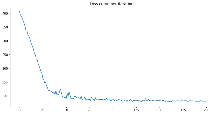
As observed with 200 iterations the minimum loss has been reached. One can experiment with the number of iterations according to the data.

Let’s now create a forecast using the fitted model. The predicted distribution across upcoming timesteps is represented by a TensorFlow Distribution instance returned by the simple call “tfp.sts.forecast.”

num_samples=120
 
pred, pred_std, forecast_samples = (
    share_forecast_dist.mean().numpy()[..., 0],
    share_forecast_dist.stddev().numpy()[..., 0],
    share_forecast_dist.sample(num_samples).numpy()[..., 0])

Particularly, the forecast distribution’s mean and standard deviation provide us with a prediction with little uncertainty at each timestep, and we can also create samples of potential futures.

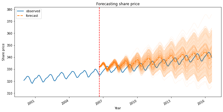
The orange part is the forecasts and the blue part is the real data. As observed the forecast deviation is increasing with time. The mean value of the forecast is represented by the dotted line.

errors_prediction=training_data-pred
errors_mean = errors_prediction.mean()
errors_std = errors_prediction.std()

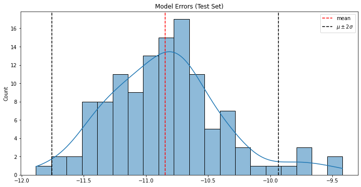
As observed with the above plot the distribution of error is highly skewed with the negative part. This means the predicted values are much higher than the observed which could also be seen in the forecast. This model definitely needs improvements. 

Conclusion

Models designed using probabilistic programming assist in decision-making in uncertain conditions. A model known as Bayesian Structural Time Series is created when the Bayesian probability is applied to structural time series. As a total of several elements, including trends, seasonal patterns, cycles, and residuals, it is expressed. With this article, we have understood the probabilistic modelling in structural time series data.

References

• Link to the above code
• Documentation on TensorFlow Probability