Tutorial on Univariate Single-Step Style LSTM in Time Series Forecasting

Long short-term memory (LSTM) in an artificial recurrent neural network(RNN) is an architecture of deep learning.

Let us take an example of any sequential data, which can be weather data or stock market data where we need to predict the weather for the next day, week, month, or the whole year. Unlike any feedforward neural network, LSTM has feedback connections. Therefore, it can predict values for point data and can predict sequential data like weather, stock market data, or work with audio or video data, which is considered sequential data.

A most common LSTM network unit consists of a cell, an input gate, an output gate, and a forget gate. A cell remembers values over an autocratic time interval. The input gate manages the flow of information coming inside of the cell. The output gate manages the flow of information going outside. Similarly, forget gates manage the flow of information that is not required or not required.  LSTM are useful for making predictions, classification and processing sequential data. We use many kinds of LSTM for different purposes or for different specific types of time series forecasting.

What is a Univariate time series?

 The term univariate implies that forecasting is based on a sample of time series data where only one factor/variable is responsible for the prediction values without considering other variables’ effects—for example, predicting the price of gold without considering the effect of marriage season in India.

In addition, we will predict only a single step value, or more formally, we can say using past values, we will predict only one value for the future. This is why the whole method can be called an LSTM univariate single step type. We will be doing forecasting analysis using LSTM models for a univariate time series with one variable changing with the time for only one future step. For this article, I am using temperature data, where the data is about the average temperature of a day observed from the year 1981 to 1990.

We will cover the following points in this article.

• EDA of time series.
• Data preparation.
• LSTM model building.
• Fitting the model and making the predictions.

Let’s start with importing the data. 

Input:

import pandas as pd

data = pd.read_excel('/content/drive/MyDrive/Yugesh/LSTM Univarient Single Step Style/temprature.xlsx', index_col = 'Date')

Here I have provided our date-time value as an index column when importing the data.

Let’s check how our data will look like.

Input:

data.head()

Output:

Let’s plot a line graph for the time series data.

Input:

data.plot(color='green')

Output:

Here we can see its cyclic data. For every year, it is almost ranging between 25-24 degrees celsius to 0-3 degrees celsius. Also, there is seasonality in the data. For more details, we should plot the line graph for two years.

Input:

data_1984 = data[(data.index>'1983-01-01') & (data.index<'1985-01-01')]

data_1984.plot(color='green')

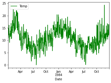
Output:

Here we can see from data between the start of 1983 to the start of 1985 wherein data the temperature value has increased three times between the months January to April and for every year in July it has touched the lowest point of temperature. By this, we can say that every year with January, the summer season starts, and around July, there is a winter season.

At this point, we should check for the autocorrelation between the values.

In time series analysis, the autocorrelation is a correlation between two consecutive points because sometimes it may happen that the previous value is affecting its future value. More formally, data points are relational.

Input:

from statsmodels.graphics.tsaplots import plot_acf, plot_pacf

plot_acf(data);

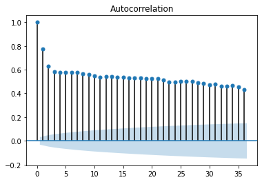
Output:

Here we can see a correlation between points lying between 0.5 to 0.6, which is quite normal. We don’t need to change anything on data( note there will always be a high correlation between starting two values)

Let’s check for partial autocorrelation also for more validation.

Input:

plot_pacf(data);

Output:

Here also we can see there is a very low partial correlation between the data points. To know more about autocorrelation and partial autocorrelation, you can go through this link.

We have seen how our time series is moving with the time next in the article; we will see how we can prepare it according to the model.

 In LSTM modeling, the model learns about the function that maps the sequence of the observations. So one thing which is necessary here is that the data should be in a proper sequence so that there will be fewer chances of loss in getting accuracy. 

Let’s consider to the following data points:

[100, 200, 300, 400, 500, 600, 700, 800, 900]

Here we can easily predict the next value because we know about the sequence; every value has the same difference to its past value, and we can say after 900, the next value would be 1000.

We can divide the sequence into multiple inputs/output patterns, considering the sample. From the division of data in the input/output pattern, the model will learn about the input patterns and the output, a  single step output, like the following – where the X is input, and the Y is output. Thus, y is one step ahead of three consecutive X values. 

     X             y

100, 200, 300    400

200, 300, 400    500

300, 400, 500    600

Here we can understand how the model function will work, and next in the article, we will prepare our data as the same as we have discussed.

Defining a function to make samples from univariate temperature sequence.

Input:

import numpy as np

def sampling(sequence, n_steps):

  X, Y = list(), list()

  for i in range(len(sequence)):

    sam = i + n_steps
    if sam > len(sequence)-1:
    break

   x, y = sequence[i:sam], sequence[sam]

    X.append(x)

    Y.append(y)

  return np.array(X), np.array(Y)

Making samples from the temperature sequence-

Input:

n_steps = 3

X, Y = sampling(data['Temp'].tolist(), n_steps)

We can also print the X and Y to understand better how our samples will look like.

Input:

for i in range(len(X)):

  print(X[i], Y[i])

Output:

Here in the brackets, our X(input) and outside in the right, our Y(output) values are rendering. We have more than 3000 values for both X and Y. That’s why I am just putting a cropped image on the output.

Defining the model.

Input:

from keras.models import Sequential
from keras.layers import LSTM
from keras.layers import Dense

model = Sequential()
model.add(LSTM(50, activation='relu', input_shape=(n_steps, n_features)))
model.add(Dense(1))
model.compile(optimizer='adam', loss='mse')

It’s a Vanilla LSTM model that has a single hidden layer in the input. So we can see that we have added 50 LSTM layers with 1 dense layer. Also, it is strongly suggested that the model is expert when the sample is provided with several features. So the function we have used to make the sample is with no. of sample and no. of time stamps. So to add no. of features in the sample data, we can simply reshape the data. Because this analysis is single step-style, I am just adding one as the no. of features in the sample.

Reshaping the X array.

Input:

X = X.reshape((X.shape[0], X.shape[1], 1))

Now the data has dimensions in [ samples, timestamp, features] format where the value of the feature is one.

Checking the summary of the model.

Input:

model.summary()

Output:

The last layer of the model, the output layer, will predict only one numeric value.

Now we can fit the data in the model.

Input:

model.fit(X, Y, epochs=200, verbose=0)

Output:

Once the model is trained, it can give the prediction.

As the sample, we need to provide the data or sample in [ samples, timestamp, features] format; we can cross-check for any three sequential temperatures or look like sequential temperatures. I am using [17, 18, 19] as my sequential temperature to predict the next timestamp temperature value.

Making an array.

Input:

x = np.array([17, 18, 19])

x = x.reshape((1, n_steps, 1))

Predicting the next value using our trained model.

Input:

ypred = model.predict(x, verbose=0)

ypred

Output:

Here we can see that the result is quite satisfying.

Conclusion

So in the article, we have seen how we can perform the EDA for forecasting analysis. We have also seen how we can make an LSTM Univariate single step-style model for time series analysis. It is useful when the situation is required to predict the future based on the last few days or events data only for the next day or any upcoming event. For example, we have just provided the temperature of the fourth day, which is based on the temperature of the last three days. For better prediction, we can increase the old days’ count or remove the noise effects from the time series. The noise is a factor that suddenly comes in the time series and increases or decreases the values of observations suddenly on the particular points. These points have increments or decrements, making it difficult to understand the model’s time series function. So we can also improve the level of accuracy by removing those noise points from the time series. 

References

• LSTM layer.
• Time Series forecasting for weather prediction.
• Google colab for codes.
• Temperature data