In time series analysis, various kinds of statistical models and deep learning models can be used for modelling purposes. Talking specifically about the deep learning models in time series, we see the huge success of the LSTM or RNN models because of their performance. In this article, we are going to discuss a model which can be built using the LSTM layers and that is a combination of two neural networks named an encoder-decoder model. We will use this model in univariate time series analysis. The Major points to be discussed in this article are listed below.

Table of Contents

1. Understanding Encoder-Decoder Model?
2. Why Encode-Decoder for Time Series?
3. Building an Encoder-Decoder with LSTM layers for Time-Series forecasting

Understanding Encoder-Decoder Model

In machine learning, we have seen various kinds of neural networks and encoder-decoder models are also a type of neural network in which recurrent neural networks are used to make the prediction on sequential data like text data, image data, and time-series data. Talking about the history of the generation of such models, they were developed to solve the machine translation problems, although these models are being used for sequential prediction problems such as text summarization and question answering.

When we talk about the architecture, we see that in the whole model, there are two recurrent neural networks. One is to encode the sequence in the input and another one is for decoding the encoded sequence into the target sequence. There are various applications where we can see the application of the encode-decoder models. Some of the applications are: 

• Machine translation 
• Text summarization 
• Image processing 
• Chatbots
• Time series forecasting

Before going deeper into the network, we should have some prior knowledge about the RNN and LSTM models. This can be obtained by using this article. Now, let’s have a look at the architecture of the encoder-decoder model.

Image source

The above image is a representation of the architecture of an encoder-decoder model. Where x is input for the model and y is the output of the model. By looking at the picture, we can say there are three main components of the architecture:

• Encoder 
• Feature vector 
• Decoder         

Encoder: It receives the elements of the input sequence one by one at every time step, learns the information from the input, and propagates it for further processes.

Feature Vector: This is an internal and intermediate state which is responsible for holding the sequential information of the input which is helpful for the decoder to make accurate predictions.

Decoder: The decoder part of the architecture can also be an RNN model which helps the model to make predictions by decoding the outcome by the encoder again in a sequential format. 

Why Encode-Decoder for Time-Series?

The time-series data is a type of sequential data which gets generated by collecting the data points obtained in a sequence with time values. When we talk about the NLP data we consider words in the data as data points and their meanings as their sequence. It becomes important to remember the sequence of the data in the NLP.  Similarly, the sequence we have in time series is important to learn to make the forecasting more accurate.  

As we have discussed in the above points, encoder-decoder models are very good with the sequential data and the reason behind this capability is the LSTM or RNN layer in the network, which are already developed to work with the sequential model. With just a finely tuned LSTM layer we can make a whole network work appropriately with the sequential information of the data by just making the network memorize the sequence. Because of the high performance with the sequential data we can use the encoder-decoder model with the time series data. 

Building an Encoder-Decoder with LSTM layers for Time-Series forecasting 

In the above section, we have discussed how the encoder-decoder model works well with the sequential information and how the time series is sequential data. This section of the article will be a representation of how we can use an encoder-decoder model for time series analysis where LSTM layers are used for making an encoder-decoder model.

Data Processing

Our first step of the section will be to imply some of the basic procedures before the modelling, like importing libraries and preprocessing the data. 

Let’s start with importing libraries.

import pandas as pd
import numpy as np
import tensorflow as tf
from sklearn import preprocessing
import matplotlib.pyplot as plt

Now let’s Importin the data set. We are using  Metro Interstate Traffic Volume data which tells about the change in the Interstate 94 Westbound traffic volume for MN DoT ATR station 301 with the temperature, rain, snow, cloud, and weather information on it.  We can extract the data from here. Let’s take a look at the 10 samples of the data.

data.head()

Output:

Let’s take a look at the description of the data.

data.describe()

Output:

Here in the above output, we can see the description of the data.

Before going to modelling we are required to perform some of the data preprocessing like removing duplicate dates from the data, splitting the data.

data.drop_duplicates(subset=['date_time'], keep=False,inplace=True)
validate = data['traffic_volume'].tail(10)
data = data.drop(data['traffic_volume'].tail(10).index)

Let’s extract traffic volume from the data.

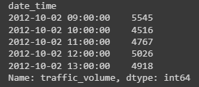
uni_data = data['traffic_volume']
uni_data.index = data['date_time']
uni_data.head()

Output:

We can make a function for preparing a univariate data as,

def custom_ts_univariate_data_prep(dataset, start, end, window, horizon):
  X = []
  y = []
  start = start + window
  if end is None:
    end = len(dataset) - horizon
  for i in range(start, end):
    indicesx = range(i-window, i)
    X.append(np.reshape(dataset[indicesx], (window, 1)))
    indicesy = range(i,i+horizon)
    y.append(dataset[indicesy])
  return np.array(X), np.array(y)

Let’s make the data univariate using the function.

  univar_hist_window = 48
horizon = 10
TRAIN_SPLIT = 30000
x_train_uni, y_train_uni = custom_ts_univariate_data_prep(x_rescaled, 0, TRAIN_SPLIT,univar_hist_window, horizon)

x_val_uni, y_val_uni = custom_ts_univariate_data_prep(x_rescaled, TRAIN_SPLIT, None,univar_hist_window,horizon)

print (x_train_uni[0])

Output:

Here we can see the single window of the past. Let’s take a look at the values in the target horizon.

print (y_train_uni[0])

Output:

In this article, we are going to use Keras provided LSTM layers for building the model which needs to transform the data according to the layers in the tensor slices.

BATCH_SIZE = 256
BUFFER_SIZE = 150

train_univariate = tf.data.Dataset.from_tensor_slices((x_train_uni, y_train_uni))
train_univariate = train_univariate.cache().shuffle(BUFFER_SIZE).batch(BATCH_SIZE).repeat()
val_univariate = tf.data.Dataset.from_tensor_slices((x_val_uni, y_val_uni))
val_univariate = val_univariate.batch(BATCH_SIZE).repeat()

Building the Model 

As we have discussed before, we use the RNN or LSTM layers to build the encoder-decoder models, and here, we are going to use LSTM layers for building models. 

# create model
from keras.models import Sequential
from keras import layer
from keras.layers import LSTM
enco_deco = Sequential()

# Encoder
enco_deco.add(LSTM(100, input_shape=x_train_uni.shape[-2:], return_sequences=True))
enco_deco.add(LSTM(units=50,return_sequences=True))
enco_deco.add(LSTM(units=15))

#feature vector
enco_deco.add(layers.RepeatVector(y_train_uni.shape[1]))

#decoder
enco_deco.add(LSTM(units=100,return_sequences=True))
enco_deco.add(LSTM(units=50,return_sequences=True))
enco_deco.add(TimeDistributed(tf.keras.layers.Dense(units=1))

Let’s compile the model.

enco_deco.compile(optimizer='adam', loss='mse')

Checking for the summary of the model:

enco_deco.summary()

Output:

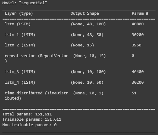
Here in summary, we can see the architecture of our encoder-decoder model. Now we are ready to fit the model on the tensors which we have prepared for modelling.   

history = enco_deco.fit(train_univariate, epochs=150,steps_per_epoch=100,validation_data=val_univariate, validation_steps=50,verbose =1)

Output:

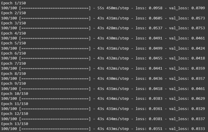
Here we have trained the model. 

Making prediction 

Now we can use the model to make predictions for the future. But before it, we are required to make the data according to the model requirement.

Let’s extract some samples from the data.

uni = df['traffic_volume']
validatehori = uni.tail(48)

Scaling and reshaping the samples:

validatehist = validatehori.values
scaler_val = preprocessing.MinMaxScaler()
val_rescaled = scaler_x.fit_transform(validatehist.reshape(-1, 1))
val_rescaled = val_rescaled.reshape((1, val_rescaled.shape[0], 1))

Now we are ready to make the prediction on the samples from the data.

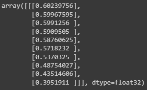
Predicted_results = enco_deco.predict(val_rescaled)
Predicted_results

Output:

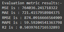
Let’s take a look at the to measure the performance of the model metrics so that we will have a measurement of the performance of the model.

from sklearn import metrics

print('Evaluation metric results:-')
print(f'MSE is : {metrics.mean_squared_error(validate,Predicted_inver_res)}')
print(f'MAE is : {metrics.mean_absolute_error(validate,Predicted_inver_res)}')
print(f'RMSE is : {np.sqrt(metrics.mean_squared_error(validate,Predicted_inver_res))}')
print(f'MAPE is : {mean_absolute_percentage_error(validate,Predicted_inver_res)}')
print(f'R2 is : {metrics.r2_score(validate,Predicted_inver_res)}',end='\n\n')

Output:

Also, we can make a graph between actual and predicted values as,

plt.plot( list(validate))
plt.plot( list(Predicted_inver_res))
plt.title("Actual vs Predicted")
plt.ylabel("Traffic volume")
plt.legend(('Actual','predicted'))
plt.rcParams["figure.figsize"] = [16,9]
plt.show()

Output:

Here we can see the performance of the model which is quite satisfactory and we can see in the graph also how the slope of the actual and predicted values are similar and values are also very similar. Adding more layers to the network can provide more beautiful results.

Final Words 

Here in the article, we have discussed an overview of the encoder-decoder model and we have discussed how it can be fruitful in time series modelling. Along with this, we have seen the implementation of the encoder-decoder model in univariate horizon style time series modelling. 

References

• Keras LSTM layers
• Link for the codes