Solving advance and complex mathematical conundrums at exascale powers supercomputing that stands at the frontiers of human advancement. Some of the architectures of supercomputing come with parallel computing capabilities over the past few decades. With ever-increasing mathematical CFD capabilities, the horizons of supercomputing are opening up.
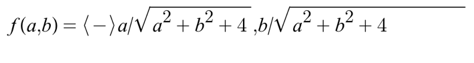
Stanford’s Engineering Center for Turbulence Research has set a world record in CFD in breaking a million-core supercomputer barrier by modelling the supersonic jet noise with 1.5 petabytes of memory with a high-speed 5-dimensional interconnect. Cray, the supercomputing company, produced a number of supercomputers during the past five decades revolutionising and solving some of the most complex and hardest vector calculus problems such as the Navier Stokes equation, invented by George Gabriel Stokes and Claude-Louis Navier. The applications of computational fluid dynamics heavily leverage vector calculus. A two-dimensional or three-dimensional vector field is a function f that maps multiple points such as (a,b) in ℝ2 , for the two-dimensional vector (x,y). A three-dimensional vector field maps the fields from (a,b,c) to (x,y,z). The two-dimensional vector field equation represented as:
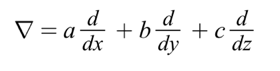
A number of data science fields leverage vectors, such as computational fluid dynamics representing different physical quantities such as gravity, electricity, velocity, and magnetism. The gradient is a critical aspect of the vector field, for the function f(a,b), the gradient can be represented as (fa(a,b), fb(a,b)). The (a,b) is the tail of the function that represents the function’s direction with maximum increase. The delta (????) operator is an important mathematical operator in vector calculus that deals with partial derivates of the vectors with differentiation and integration over the vector fields. If we consider, a,b,c as the unit vectors for the coordinate axes, the delta operator represented as:
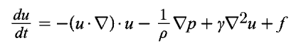
Navier Stokes equations are implemented on CFD (computational fluid dynamics) by the supercomputers for compressible and incompressible flow. Cray XMP and 205 implemented Navier Stokes and Euler’s equations with three-dimensional configurations. The Navier Stokes equations applied to solve many of the complex problems for simulating a physical phenomenon such as smoke or fire as an application of Newton’s second law, F = ma, represented as the product of the acceleration of the object and mass of the object. We can represent f as the forces and leverage density and shear stress. The density denoted as the measurements of the object’s mass per unit volume and shear stress can be defined as the stress coplanar component as:

where;
p: Density of the fluid and the equivalent of the density to mass
????: Velocity

????: Shear stress
f: Forces
????. ???? + f: Total force
The above equation can also be represented as:

where;
P: Pressure
????: Dynamic viscosity
Dividing the pressure p and subtracting the ????. ???? u, we can derive the traditional form of the Navier-Stokes equation.
Fluid-dynamic resonance is excited by the thin boundary layers in compact cavities around the periphery of mirror casings, predicting cavity and local flow conditions. The Navier-Stokes equation can solve in 2-dimensions with different boundary conditions. The differential equations for cavity flow for velocity components ????, v can be represented as:
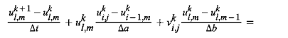
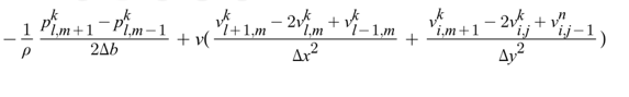
Leveraging applied mathematics, we can discretise the ???? dynamic viscosity momentum-equation as follows by transferring the equations into discrete parts for numerical evaluations and further implementation in PyTorch or Python in machine learning.

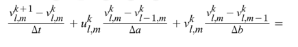
We can also discretise v, the viscosity measurements of resistance another type of momentum equation as follows:
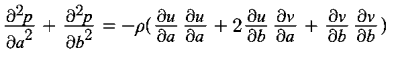
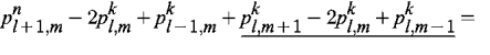
The pressure Poisson equation for incompressible Navier-Stokes equation can be written as a solver with Neumann boundary conditions with discretisation.

George Gabriel Stokes introduced the Reynolds numbers (Re), a quantity in computational fluid mechanics that provides the ratio between inertial forces to viscous forces. It represents:
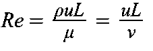
ρ à Density of the fluid
u à Speed of the flow
L à Linear dimension
???? à Dynamic viscosity of the fluid
ν à The measure of resistance to the flow of a fluid
The distributeddataparallel can be leveraged in PyTorch to implement the data parallelism at each module level for distributed high-performance and supercomputing with collective communications in the torch.distributed package by synchronising the buffers and gradients across clusters and processes of machines with different communication strategies for point-to-point communications. Especially, when there is a large number of data points in computational fluid dynamics (CFD), the deep neural networks require large-scale compute and hardware on clusters of machines. Massive parallel computing capabilities with both forward and backward pass with parallelism on GPUs need distributed supercomputing. The minibatch stochastic gradient algorithm can be applied to train the deep neural networks across the batch by scaling the learning rate and hyperparameter tuning for improved performance. The parallelising techniques either on PyTorch or TensorFlow, involve the following steps primarily.
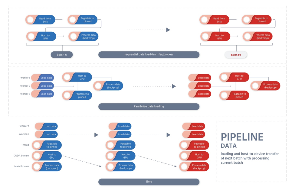
Loading the data from the disk into the host, leveraging multi-threading for data parallelisation from the pageable memory to the host’s pinnable memory. As soon as the data gets loaded from the disk into the main memory and gets transferred from the GPU’s pinnable memory, the calculation of gradients with the backward pass and forward pass occurs, and the parameters get updated in a highly computer-intensive parallel task with multiple computations. Dataloader is a framework, which is a class in PyTorch that takes the dataset as the argument by loading the data from the disk and from pageable to pinnable memory. Data pipelines significantly scale up parallelised and pipelined data loading instead of the serial data loading.