Listen to this story

Classification accuracy is a statistic that describes a classification model’s performance by dividing the number of correct predictions by the total number of predictions. It is simple to compute and comprehend, making it the most often used statistic for assessing classifier models. But not in every scenario accuracy score is to be considered the best metric to evaluate the model. In this article, we will discuss the reasons not to believe in the accuracy performance parameter completely. Following are the topics to be covered. 

Table of contents

1. About Classification
2. About Classification accuracy
3. Scenarios where accuracy fails
4. Alternatives for accuracy
5. Example of accuracy failure

Let’s start with understanding the failure of the accuracy parameter to capture the actual performance of the machine learning algorithm.

About Classification

The Classification method is a Supervised Learning approach that uses training data to identify the category of fresh observations. The algorithm in Classification learns the pattern from a given dataset or observations and then classifies additional observations into one of many classes. Classes can also be referred to as targets/labels or categories.

In contrast to regression, the outcome variable of Classification is a category rather than a continuous value, such as “Yes or no”, “0 or 1”, and so on. Because the Classification method is a Supervised learning approach, it requires labelled input data, which implies it comprises input and output.

Are you looking for a complete repository of Python libraries used in data science, check out here.

About classification accuracy

Predicting a class label from instances in a problem area is what classification predictive modelling is all about. Classification accuracy is the most frequent parameter used to assess the effectiveness of a classification prediction model. Because the accuracy of a predictive model is often high (over 90%), it is usual to characterise the model’s performance in terms of the model’s error rate.

Classification accuracy is achieved by first employing a classification model to predict each sample in a test dataset. The predictions are then compared to the known labels for the test set examples. Accuracy is then determined as the proportion of accurately predicted examples in the test set divided by all predictions made on the test set.

Accuracy= Correct  predictions/Total  predictions

In contrast, the error rate may be computed by dividing the total number of inaccurate predictions made on the test set by the total number of predictions made on the test set.

Error rate= Incorrect  predictions/Total  predictions

Since accuracy and error rate are complementary, they could always be computed one from the other.

Accuracy = 1- Error rate
Error rate = 1- Accuracy

Scenarios where accuracy fail

When the distribution of instances to classes is skewed, then accuracy fails to capture the actual performance of the algorithm. 

Consider a binary unbalanced dataset with a class imbalance of 1:100 which means for every case of the minority class, there will be 100 examples of the majority class.

In this sort of challenge, the majority class symbolises “normal,” while the minority class represents “abnormal,” such as a flaw, or a fraud. A strong performance in the minority class will be chosen above a strong performance in both groups.

A model that predicts the majority class for all cases in the test set will have a classification accuracy of 0.99, matching the average distribution of major and minor examples in the test set.

Many machine learning models are built on the premise of balanced class distribution, and they frequently learn basic rules that are either explicit or implicit. It’s the same as always predicting the majority class, resulting in an accuracy of 0.99, but in practice doing no better than an untrained majority class classifier.

The accuracy reports a correct result; the point of failure is the practitioner’s perception of high accuracy ratings. Instead of rectifying incorrect intuitions, different measures are commonly used to characterise model performance for unbalanced classification issues.

Alternatives for accuracy

The objective of evaluating classification models is to determine how closely the classification recommended by the model corresponds to the actual categorization of the case. There are several measures for evaluating the model’s performance depending on the technique of observation.

Confusion Matrix

A confusion matrix is not a measure for evaluating a model, but it does give information about the predictions. It is necessary to understand the confusion matrix in order to understand other classification metrics such as accuracy and recall.

The confusion matrix goes beyond classification accuracy by displaying the accurate and wrong (i.e. true or false) predictions for each class. A confusion matrix is a 2×2 matrix in the case of a binary classification problem. If there are three separate classes, the matrix is 3×3, and so on.

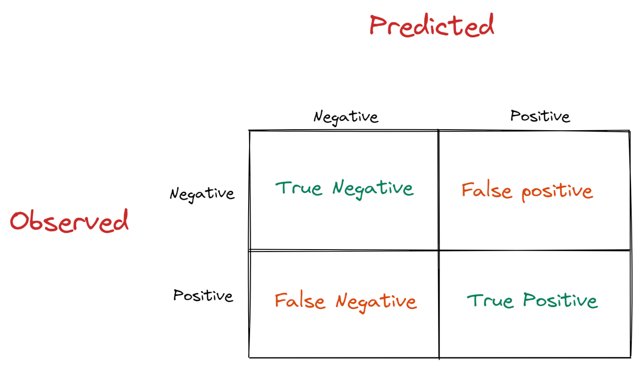
• True Negative (TN) is the proportion of valid forecasts that are negative
• False Positive (FP) is the frequency of inaccurate guesses that occur in positive cases 
• False Negative (FN) is the number of inaccurate guesses that occur in bad situations 
• True Positive (TP) is the frequency of positive examples with correct forecasts

Precision and Recall

Precision is the proportion of positive events that are genuinely positive. It assesses “how helpful the classifier’s results are.” Precision assesses how accurate our model is when the forecast is correct.

Precision=True Positive/(True Positive + False Positive)

Otherwise, a precision of 90% means that when our classifier flags a customer as fraud, it is truly fraud 90% of the time. Positive forecasts are the emphasis of precision. It shows how many optimistic forecasts have come true.

Another approach to look at the TPs is via the lens of recall. Recall is the proportion of true positive events that are marked as such. It assesses “how complete the outcomes are,” or what percentage of real positives are projected to be positive.

Precision=True Positive/(True Positive + False Negative)

Actual positive classifications are the objective of recall. It reflects how many of the positive classifications the model accurately predicts.

ROC Curve and Area Under the Curve (AUC)

The ROC graph is another method for evaluating the classifier’s performance. The ROC graph is a two-dimensional graphic that shows the false positive rate on the X axis and the true positive rate on the Y axis.

In many situations, the classifier includes a parameter that may be modified to increase genuine positive rates at the expense of raising false positive rates or to decrease false positive rates depending on the declining value of actual positive rates. Each parameter setting provides a par value for a false positive rate and a positive actual rate, and the number of such pairings may be utilised to describe the ROC curves. The following are the characteristics of a ROC graph.

• The ROC curve or point is independent of the class distribution or the cost of mistakes.
• The ROC graph comprises all of the information included in the error matrix.
• The ROC curve is a visual tool for measuring the classifier’s ability to properly identify positive and negative examples that were mistakenly categorised.

In many situations, the area under the one ROC curve may be employed as a measure of accuracy, and it is known as measurement accuracy based on the surface.

Example of accuracy failure

Let’s have a look at when the accuracy performance parameter fails to capture the actual performance on a dataset.

import pandas as pd
import numpy as np
import matplotlib.pyplot as plt
import seaborn as sns
 
from sklearn.linear_model import LogisticRegression
from sklearn.metrics import accuracy_score,precision_score,recall_score,plot_confusion_matrix,confusion_matrix
from sklearn.model_selection import train_test_split
 
import warnings 
warnings.filterwarnings('ignore')

Reading the data, preprocessing

df=pd.read_csv('https://raw.githubusercontent.com/analyticsindiamagazine/MocksDatasets/main/healthcare-dataset-stroke-data.csv')
df_utils=df.dropna(axis=0)
df_utils[:8]

df_new=pd.get_dummies(df_utils,drop_first=True)
df_new.shape

Encoding all the categorical values for the learner. Let’s analyse the target column and check the balance of the data.

sns.countplot(df_utils['stroke'])
plt.show()

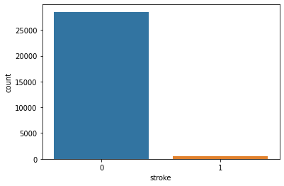
This plot clearly shows that the data is highly imbalanced. Let’s fit our logistic regression learner and check the performance of this data.

X=df_new.drop('stroke',axis=1)
y=df_new['stroke']
X_train, X_test, y_train, y_test = train_test_split(X, y, test_size=0.30, random_state=42)

lr=LogisticRegression()
lr.fit(X_train,y_train)
y_pred=lr.predict(X_test)
accuracy=np.round(accuracy_score(y_test,y_pred),2)
precision= np.round(precision_score(y_test,y_pred),2)
recall= np.round(recall_score(y_test,y_pred),2)

So, the scores say that our model has performed very well as the accuracy score is 0.95, the precision is 0.50 and the recall is 0.01. Let’s compare the test and prediction with the help of a plot.

fig, axes = plt.subplots(1, 2, figsize=(10,5))
sns.countplot(y_test,ax=axes[0])
axes[0].set_title('observed')
sns.countplot(y_pred,ax=axes[1])
axes[1].set_title('predicted')
plt.show()

But the plot tells a difference: the learner predicted a negligible amount of ‘1’s. This is due to the fact that the data was imbalanced. Let’s use a resampling technique to mitigate this problem. 

In this article, we are going to use the oversampling method known as  Synthetic Minority Oversampling Technique (SMOTE). This practise produces duplicate instances in the minority class, despite the fact that these examples provide no new information to the model. Instead, new instances may be created by combining old ones.

from imblearn.over_sampling import SMOTE
smt = SMOTE(k_neighbors=5, random_state=42)
X_train_res, y_train_res = smt.fit_resample(X_train, y_train)
 
print('After SMOTE, the shape of train_X: {}'.format(X_train.shape))
print('After SMOTE, the shape of train_y: {} \n'.format(y_train_res.shape))
 
print("After SMOTE, counts of label '1': {}".format(sum(y_train_res == 1)))
print("After SMOTE, counts of label '0': {}".format(sum(y_train_res == 0)))

Here it could be observed that the total number of data points is been balanced in both the categories (0,1).

Let’s plot a comparison between before and after resampling.

From the plot, we can observe that the resampling technique worked and the minority class was resampled. We will be only resampling the training part because this part will be used for training and the test part should always be unchanged. 

lr_res=LogisticRegression()
lr_res.fit(X_res,y_res)
y_pred_res=lr_res.predict(X_test)
accuracy_res=np.round(accuracy_score(y_test,y_pred_res),2)
precision_res= np.round(precision_score(y_test,y_pred_res),2)
recall_res= np.round(recall_score(y_test,y_pred_res),2)

Now all the scores are being stored, create a dataframe to store the before and after results of the resampling so that we can have a better understanding of the variations.

df_scores=pd.DataFrame([[accuracy, precision,recall], [accuracy_res, precision_res, recall_res]],
              index=['before', 'after'],
              columns=['accuracy', 'precision','recall'])
df_scores

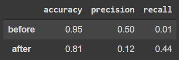
There is a difference in the accuracy score of the model and from 0.95 it has fallen down to 0.81, and the recall score has increased.  

Conclusions 

Accuracy and error rate is the standard measures for characterising classification model performance. Because practitioners built intuitions on datasets with an equal class distribution, classification accuracy fails on classification tasks with a skewed class distribution. With this hands-on article, we have understood that high accuracy in classification problems is not always better. 

References

• Link to the above code
• Know more about the evaluation of classification