Visualising an object in 4D is nearly impossible, but mathematically, can be defined. For example, let’s say there are certain data related to weather of a city consisting of attributes like temperature, air pressure, humidity, wind speed and time of day. In a feature space, these five attributes can be viewed as to be in a 5-dimensional space. A typical plot (time vs pressure, time vs temperature, etc) is the “shadow” of that hypersurface. The shadow of a 4-dimensional hypercube or the tesseract can be imagined to be projected as a cube.

Every n-cube of n > 0 is composed of elements, or n-cubes of a lower dimension, on the (n−1)-dimensional surface on the parent hypercube. A side is an element of (n−1)-dimension of the parent hypercube. A hypercube of dimension n has 2n sides.

A recent study by by Bren Daniel and E Young, tries to open up new avenues in the field of topology. The complexity of a neural network increases with increasing depth of the network. The edges of a hypercube, with its multi-dimensional feature, can be interpreted as the connections between the hidden layers or even in simpler terms, a multi-dimensional decision trees. These analogies partially make sense because 4D visualisation is not intuitive.

A Quick Recap Of One-Shot Learning

One shot learning is devised to teach the machine to learn the human way. Just as humans learn about the objects and notice the attributes with whatever little information is available and then later, identify a similar object. So, a technique to train the models on minimum information or labelled data. One-shot learning differs from single object recognition and standard category recognition algorithms in its emphasis on knowledge transfer, which makes use of prior knowledge of learnt categories and allows for learning on minimal training examples.

Constructive Training of Neural Network

One or more topological covering maps are defined between a network’s desired input and output spaces; these covering spaces are encoded as a series of linear matrix inequalities; and, finally. The series of linear matrix inequalities is translated into a neural network topology with corresponding connection weights.

Imagine the case where an input dataset has three dimensions: each piece of input data could be represented as a point in 3D space where each point is a category. Imagine a cube containing all such points, and the cube itself is fragmented into many tiny cubes of the same size. If these tiny cubes were sufficiently small, then each cube would only contain points belonging to a single category (sufficiently small cubes would only contain a single point, making this trivially true). Each cube is assigned a category to classify a new point,

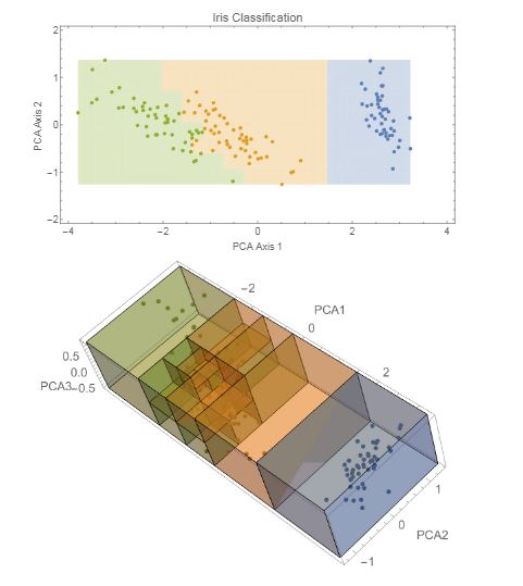
The bisection algorithm is able to achieve roughly 96% accuracy when using two, three, or four PCA directions as compared to the roughly 75% mean accuracy achieved by a traditionally trained neural network.

For the purposes of comparison here, many different topologies were explored ranging from 8 to 128 nodes in each of between one and three hidden layers.

All reported accuracies were extracted from a network with a single hidden layer of 32 nodes.

In this study, evaluation accuracy appeared to depend far more strongly on the randomized weights initially assigned to the network than on the training time provided to it.

The bisection algorithm simply runs to a deterministic completion, i.e. , to the point that all training data are correctly classified, or a minimal scale has been reached, removing the ambiguity surrounding training time. A similar comparison was made using wine data set and MNIST datasets too.

Check the full algorithm and experimental procedure here.

Key Takeaways

• Specifying the shape and depth of a neural network using topological covering.
• Using two design variables – unit cover geometry and cover porosity for cover-constructive learning.
• Using a constructive algorithm to train deep neural network classifier in one shot.

This algorithm is the first in a new class of algorithms for constructive deep learning; future work will investigate the Reeb graph and Morse theory methods for data shape decomposition and neural network parameterization. MNIST and IRIS datasets used for this experiment showed decent results. But, the real question is whether this new constructive learning will outrank the traditional methods eventually.